


0 Introduction
Tomatoes are a crucial crop, renowned for their high nutritional and health value, providing essential vitamins and trace elements. They also hold significant economic value due to their widespread global cultivation[1]. Accurate and real-time monitoring of tomato growth and yield is essential for optimizing production, planning export, and evaluating yield-enhancing measures. Existing methods for monitoring and predicting tomato growth primarily include empirical models, mechanistic models, semi-empirical semi-mechanistic models, machine learning models, and deep learning models.
The study of tomato growth models is a vital component of crop modeling. Previous explorations of in this field have categorized based on their establishment methods into mechanistic, semi-mechanistic, and empirical models. Mechanistic models involve mathematical descriptions of plant processes based on known plant mechanisms and are simulated theoretically. Empirical models rely on statistical regularities to study crop growth. Semi-mechanistic models represent a fusion of these two approaches[2]. Typical mechanistic models include TMOGRO[3] and TOMSIM, which use a series of equations to reflect the impact of environmental variables— such as indoor temperature, CO2 concentration, and light on crop growth, morphological changes, and dry matter accumulation. While mechanistic models offer an accurate mathematical depiction based on theoretical simulation, the complexity of actual physiological processes introduces uncertainties and errors that require further investigation[4]. Empirical models, such as those based on dry matter allocation coefficients, derive parameters through estimation and fitting based on statistical regularities, ensuring model accuracy. Compared to mechanistic models, empirical models are more accessible and widely applicable, with strong practical value. Mechanistic models, while addressing immediate problems, also allow for more in-depth research and exploration, holding significant theoretical value.
The integration of machine learning with crop models has experienced rapid development, falling within the realm of empirical models and showcasing strong practicality. In the early stages of this integration, research predominantly focused on the application of BP neural networks. Han et al.[5] successfully developed a principal component analysis-backpropagation neural network (PCA-BPNN) network to predict fruit diameter based on air temperature, air humidity, soil moisture content, and leaf temperature, achieving a maximum error of only 0.075 mm. Focusing on flowering tomatoes, Zhang et al.[6] established a prediction model for environmental factors and photosynthetic rate using a BP network. The models fitted under various conditions achieved a high accuracy, with an R 2 value of 0.96 between the highest predicted and actual values. Additionally, BP network-based models have been successfully applied in predicting winter wheat water consumption[7], conducting comprehensive evaluation of soil nutrient models[8], and modeling CO2 concentration models for the growth of shiitake mushrooms[9]. All these applications have yielded promising results, highlighting the potential of machine learning in agricultural modeling. Deep learning has revolutionized the integration of machine learning with crop models, particularly through advanced image processing and the incorporation of environmental data. By leveraging deep networks and convolutional methods, deep learning achieves high accuracy in crop growth analysis. For instance, Chen et al.[10] combined structural and near-infrared image features, identifying random forest as the optimal approach for biomass prediction. Yang et al.[11] used convolutional neural network (CNN) with random forests and depth maps, thereby reducing the normalized mean square error (NMSE) in lettuce growth predictions. Chandel et al.[12] demonstrated that GoogleNet excelled in classifying water stress, while Yalcin[13] used activation maps derived from sunflower images for yield estimation. Beyond image analysis, deep learning also excels when working solely with environmental data. Bali et al.[14] showed that long short-term memory (LSTM) models outperformed other methods in predicting wheat yield using historical climate data. Nigam et al.[15] assessed various deep learning models for yield prediction based on temperature and rainfall. Elavarasan and Vincentt[16] achieved 93.7% accuracy in crop yield prediction with a Q-network model. In tomato yield prediction, De Alwis et al. [17] proposed a domain adaptation long short-term memory (DA-LSTM) model that outperformed traditional LSTM, XGBoost Regression (XGBR), and support vector regression (SVR) models. Zhou et al.[18] integrated the TOMSIM and GreenLight models with deep neural network(DNN) to improve predictions of greenhouse climate-tomato production. Statistics revealed a 30-fold increase in the use of deep learning for crop yield prediction from 2016 to 2020[19], often surpassing the performance of traditional models[20]. However, deep learning's reliance on specific datasets limits its transferability between different crops or regions[21, 22], necessitating extensive localized data to address regional variation and ensure model adaptability.
In recent years, research on plant growth prediction utilizing multi-modal data has predominantly centered on remote sensing information. For instance, Maimaitijiang et al. [23] integrated RGB, multispectral, and thermal sensors within a DNN framework to predict soybean grain yield. Their findings indicated that multi-modal fusion within the DNN framework yields relatively stable and reliable prediction results. Similarly, Yang et al.[24] leveraged multi-source remote sensing data alongside non-remote sensing data (such as temperature and precipitation) to estimate key growth parameters—leaf area index (LAI), aboveground biomass (AGB), leaf nitrogen content (LNC), and soil plant analysis development (SPAD) values—during the early growth stage of canola seedlings. By comparing various model frameworks, including SVR, partial least squares (PLS), BPNN, and neural matrix regression (NMR), they found that models integrating multi-source remote sensing and non-remote sensing data achieved the highest average accuracy. Further advancing this field, Lin et al.[25] proposed a deep learning model based on multi-modal fusion, utilizing RGB-D images to automatically estimate the fresh weight of lettuce seedlings. The model achieved a root mean square error (RMSE) of 25.3 g and an R² of 0.938 across the entire growth period of lettuce, demonstrating the significant enhancement in prediction accuracy afforded by multi-modal fusion across different growth stages. However, the reliance on remote sensing data is not without limitations. Such data may result in the loss of fine-grained details and is primarily suited for large-scale predictions. Moreover, the use of multispectral and RGB-D data introduces challenges related to convenience and usability, which can hinder practical application. Certainly, there are also simple, user-friendly multi-modal models capable of performing various predictions, such as large language models (LLMs)[26]. In this study, a deep learning model was employed as a baseline model for comparative analysis. Building upon this foundation, multi-modal data were employed to develop high accuracy models for predicting tomato growth height. Environmental signals, including light and temperature, with specific plant conditions and growth-stage images were entegrated to track plant development. This method effectively synthesizes both phenotypic and temporal features, providing a comprehensive understanding of the interaction between tomato plants and their environment, thereby improving prediction accuracy. A key innovation of this work lies in the use of simple RGB images combined with sensor data, coupled with individualized monitoring of each plant. This approach enables to the capture of more detailed growth phenotype information, resulting in a more granular and precise model for plant growth prediction, which contrasts with the challenges faced by larger-scale, remote sensing-based approaches.
1 Materials and data
1.1 Study setup
The study was conducted from May 1, 2023, to July 1, 2023, in a greenhouse located at the Horticulture Division of the Heilongjiang Academy of Agricultural Sciences. The greenhouse, oriented east-west, measures 40 m in length, 40 meters in width, with a roof ridge height 6 m and eaves height of 4.5 m. Sixteen rows of tomatoes were cultivated, organized into seven groups, including four control groups. The total planting area covered 15 m2, and the tomato varieties used were Guanghui 201 and Jinzhu. A total of 78 plants were continuously monitored for growth and utilized as training data. Standard horticultural practices such as pruning side shoots and removing lower leaves, were consistently applied throughout the growth process. The Japanese Yamazaki nutrient solution (tomato-specific) formula, detailed in Table 1, served as the foundation for fertilization. Fertilization was administered every 15 days after planting, with the control group (CK) receiving 27.2 g of KH2PO4, 52.3 g of K2SO4, and 4.4 g of CaCl2 per application.
Table 1 Comparison on fertilization methods of different tomato groups |
| KNO3/g | NH4H2PO4/g | KH2PO4/g | K2SO4/g | MgSO4·7H2O/g | CaCl2/g | CaNO3·4H2O/g | |
|---|---|---|---|---|---|---|---|
| CK | 0.0 | 0.0 | 27.2 | 52.3 | 24.6 | 44.4 | 0.0 |
| T1 | 13.4 | 7.7 | 0.0 | 34.8 | 24.6 | 44.4 | 0.0 |
| T2 | 26.9 | 7.7 | 0.0 | 17.4 | 24.6 | 44.4 | 0.0 |
| T3 | 40.4 | 7.7 | 0.0 | 0.0 | 24.6 | 44.4 | 0.0 |
| T4 | 40.4 | 7.7 | 0.0 | 0.0 | 24.6 | 29.6 | 11.8 |
| T5 | 40.4 | 7.7 | 0.0 | 0.0 | 24.6 | 14.8 | 23.6 |
| T6 | 40.4 | 7.7 | 0.0 | 0.0 | 24.6 | 0.0 | 35.4 |
The trace elements are applied according to the Table 2.
Table 2 Micronutrient application of tomato |
| Molecular | Molecular weight standard concentration/(mg/L) |
|---|---|
| FeSO4·7H2O | 13.206 |
| EDTA·H2O | 17.679 |
| EDTA·3H2O | 20.000 |
| MnSO4·H2O | 1.614 |
| MnSO4· 4H2O | 2.130 |
| H3BO3 | 2.860 |
| ZnSO4·7H2O | 0.220 |
| CuSO4·5H2O | 0.080 |
| Na2MO4·2H2O | 0.020 |
1.2 Data collection
1.2.1 Automatic data collection
The greenhouse was equipped with sensors to measure air temperature, air humidity, soil temperature, soil humidity, light intensity, and carbon dioxide levels. Environmental data was automatically collected at 30-minute intervals. Additionally, a high-resolution camera, positioned directly above the monitored crops, captured images at 8:00 AM, 10:00 AM, 2:00 PM, and 4:00 PM daily. Each camera covered a designated area, capturing images of 12 plants. These images were subsequently segmented into uniform sizes and used as training data for the study.
1.2.2 Manual data collection
Certain plant growth data not captured by sensors were manually collected on a weekly basis. These included leaf area, leaf angle, plant height, normalized difference vegetation index (NDVI), ratio vegetation index (RVI), leaf nitrogen content (LNC), leaf nitrogen accumulation (LNA), LAI, and leaf dry weight (LDW). Leaf area was calculated by multiplying the distance from the stem to the top of the leaf at its widest point, derived through fitting. Leaf angle was measured using a protractor, while plant height was determined by measuring the distance from the ground to the top bud using a tape measure. NDVI, RVI, and related data were acquired using the TOP-1200 Crop Canopy Analyzer. Data collection for leaf area, leaf angle, and plant height was conducted weekly from May 7 to June 17, whereas NDVI, RVI, and related data were collected weekly from May 21 to June 17. For clarity and convenience in the following discussions, image data will be referred to as phenotypic data, while automatically collected structured environmental data and manually measured plant morphological parameters will be referred to as temporal data. However, it should be noted that phenotypic data inherently includes the measured plants parameters.
Overall, the constructed dataset included 4 368 single-plant images of 78 plants collected over a 56-day period from May 7 to July 1. Additionally, it contained 624 measurement records of plant height, leaf area, and leaf angle, collected across 8 weekly groups, as well as 468 records of plant growth indicators such as NDVI and RVI, collected across 6 weekly groups.
2 Methods
The proposed method utilizes multi-modal data to capture both phenotypic and temporal relationships, which are essential for accurate tomato growth height prediction. Specifically, the method integrates phenotypic features extracted from plant images with temporal patterns derived from environmental factors, such as light and temperature, over time. The key stages of the method include data preprocessing, network training, and performance evaluation. During training, a CNN extractes phenotypic features from the images, while a LSTM captures temporal dependencies within the environmental data. By aligning these two types of features in a joint space, the model achieves comprehensive spatiotemporal fitting, significantly enhancing its ability to model the dynamic interactions between the plant and its environment.
2.1 Data preprocessing
The collected raw data contained some missing plant data, and feature extraction was required for the image data. Therefore, data preprocessing was an essential step to ensure data quality and usability.
2.1.1 Handling missing data
During the experiment, some plants died, resulting in missing subsequent growth data. Although growth data during their survival period were recorded, these instances were excluded from the dataset due to the abnormal growth conditions observed during their lifespan and their premature death. These exclusions were implemented by filtering out records associated with plants that did not complete the entire experimental period. As a result, only complete growth data under stable conditions were retained for analysis, ensuring the reliability and consistency of the dataset.
2.1.2 Data imputation using interpolation
Due to varying sampling intervals for different data types, data alignment was necessary. The data were aligned on a daily basis, with sensor and image data recorded at fixed times each day to minimize interference from external variables. For manually measured data at weekly intervals, linear interpolation was applied to fill in missing values. Similarly, NDVI, RVI, and related data from May 7 to May 20, where data were missing, were also imputed using linear interpolation. Linear interpolation can be expressed as Equation (1) and Equation (2) .
Where, L(m,b) is the loss function to be minimized; n is the total number of weeks of the data; wi is the current number of weeks; i is the index representing the specific week, m and b are the two parameters of the linear regression model, representing the slope and intercept, respectively, The final interpolation value is represented by vi .
2.2 The training networks and evaluation metrics
CNNs are highly effective for computer vision tasks. A basic CNN structure typically consists of a convolutional layer, a pooling layer, and a fully connected layer, as illustrated in Fig. 1. The CNN processes the original image, extracting features to generate a feature map. More complex CNNs involve multiple convolution and pooling operations, often enhanced by activation functions, to improve performance. CNNs, whether used independently or as part of hybrid models, are widely employed for feature extraction in crop images[27-29]. In this study, a multi-layer CNN architecture was utilized to capture complex phenotypic patterns in tomato images, extracting high-level visual features that correlated with growth morphology.
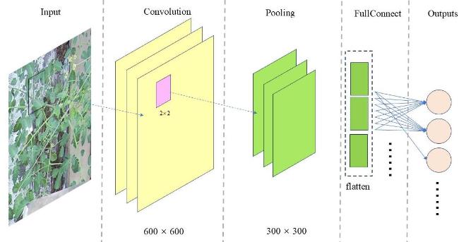
Fig. 1 Architecture of simple CNN |
Recurrent neural networks (RNNs) excel in learning from sequential data. They incorporate an additional hidden layer to retain information from previous inputs, updating the hidden layer at each step based on the current result. However, RNNs can suffer from the issue of fading long-term memory. LSTM networks address this limitation by introducing a long-term memory chain, which is particularly advantageous for predicting tomato growth. This capability allows the model to capture long-term dependencies in daily environmental changes and their impact on growth. Both RNNs and LSTMs have demonstrated effectiveness in establishing crop morphology models. The schematic diagrams of RNN and LSTM structures are illustrated in Fig. 2.
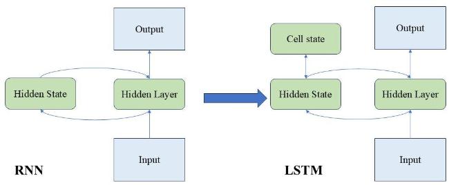
Fig. 2 Architecture of RNN and LSTM |
The CNN-RNN and CNN-LSTM architectures were employed to model tomato growth morphology. To evaluate the effectiveness of these models, metrics such as accuracy, precision, recall, and F 1-Score were utilized. The results were compared to identify the most effective model configuration for capturing tomato growth dynamics. These metrics provided a comprehensive assessment of each model's ability to generalize spatiotemporal patterns in multi-modal data, underscoring the potential of the CNN-RNN and CNN-LSTM models for intelligent, data-driven crop management.
2.3 Research framework
The process flow is illustrated in Fig. 3. The proposed approach, based on the phenotypic feature extraction (PFE) method, begins by collecting two primary types of data: Plant images and environmental measurements. These data sources undergo an initial preprocessing step, where the raw inputs were cleaned, aligned, and prepared for further analysis to ensure data consistency and reliability.
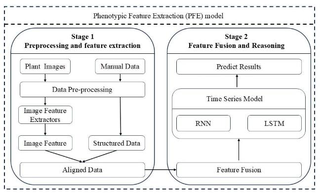
Fig. 3 Process flow of tomato growth height prediction method by phenotypic feature extraction using multi-modal data study |
Following preprocessing, the aligned image data was processed through phenotypic feature extractors within the PFE framework, capturing critical phenotypic patterns and characteristics from the images. Simultaneously, the structured environmental data was integrated into the pipeline. These phenotypic features and structured data were then fused to create a unified feature representation that combines visual and contextual environmental information.
Next, this unified representation was transformed into phenotypic-temporal features, a hallmark of the PFE method, by embedding phenotypic information extracted from images and temporal patterns derived from sequential data. Temporal feature extractors were then applied to these phenotypic-temporal features, enabling the capture of dynamic temporal relationships that reflect the evolution of plant growth over time.
By leveraging the PFE approach, this comprehensive pipeline achieved a rich representation of the plant growth process, effectively integrating both visual and environmental data to enhance the model's predictive accuracy and robustness.
2.4 Experimental setup
Original images, each containing 12 plants per group, were processed and segmented into individual plants images of size 600×600 pixels. A CNN was employed to extract feature vectors from these segmented images. The detailed network structure and parameters of the CNN are provided in the Table 3.
Table 3 Parameters for CNN operation of extract image features |
| Network Structure | Parameters |
|---|---|
| Convolutional kernel | 3×3 |
| Convolutional stride | 1 |
| Convolutional padding | 1 |
| Pooling kernel | 2×2 |
| Pooling stride | 2 |
| Fully connected input | 16×300×300 |
| Fully connected output | 16 |
The features extracted by CNN were concatenated with other temporally interpolated features. The resulting multi-modal feature vector had a size of 1×34, structured as {[treatment, variety, leaf area, height, LNC, air temperature, relative humidity, light, CO2, soil moisture, soil temperature, KNO3, NH4H2PO4, KH2PO4, K2SO4, MgSO4·7H2O, CaCl2, CaNO3·4H2O] + image feature vector (1×16)}. To ensure fair comparisons and avoid bias due to varying data magnitudes, all data were normalized to the range [0, 1].
3 Results and analysis
In the training dataset, the leaf area data on the first day (Mean = 208.2, Standard deviation = 68.14, Coefficient of variation(CV) = 32.7%) and plant height data (Mean = 18.6, Standard deviation = 3.1, CV = 16.7%) exhibited a relatively concentrated distribution. In contrast, on the last day, the leaf area data (Mean = 3 113.7, Standard deviation = 1 050.5, CV = 33.7%) and plant height data (Mean = 186.8, Standard deviation = 49.23, CV = 26.3%) demonstrated significantly greater variability. Notably, the standard deviation of the leaf area reached 1 050.5, indicating that leaf area is an unstable metric and may not serve as a reliable indicator of plant growth status. Although plant height was relatively more stable compared to leaf area, its CV increased from 16.7% to 26.3% (CV > 20%), suggesting potential instability in the dataset overall.
However, the training dataset comprised two distinct plant varieties. When analyzing the plant height data of these two varieties separately on the last day, Guanghui 201 exhibited a mean of 149.7, a standard deviation of 29.3, and a CV of 19.5%, while Jinzhu showed a mean of 223.8, a standard deviation of 35.2, and a CV of 15.7%. These CV values fall within an acceptable range, and the variability in plant height decreases when analyzed separately by variety. These variations in leaf area and plant height suggest that the features may influence the accuracy of tomato growth height prediction. Specifically, while leaf area exhibits higher variability and is less stable, plant height shows more stability and can serve as a more reliable predictor. The increased CV in plant height over time indicates some fluctuation that could impact the long-term prediction accuracy. This analysis suggests that integrating both features (leaf area and plant height) into the prediction model, with an emphasis on plant height as a key feature, may enhance the robustness of the growth height prediction, particularly when accounting for the variability across different growth stages.
3.1 RNN temporal prediction and model hyperparameter selection
The performance of the RNN network was evaluated for short-term, medium-term, and long-term temporal predictions. Three training scenarios were considered: Predicting the next 2 days based on the past 5 days (Hereafter referred to as "short-term prediction"), predicting the next 4 days based on the past 10 days(Hereafter referred to as "mid-term prediction"), and predicting the next 12 days based on the past 30 days(Hereafter referred to as "long-term prediction"). The RNN network structure parameters are detailed in Table 4. The dataset was split into training, validation, and test sets in an 8:1:1 ratio.
Table 4 Parameters for RNN operation of tomato height prediction |
| Network structure | Parameters |
|---|---|
| Input features | 34 |
| RNN hidden size | 30 |
| RNN layers | 2 |
| Learning rate | 0.001 |
| Loss function | MSELoss |
| Optimizer | Adam |
|
The input feature dimension was 34, representing the concatenation of environmental factors and image-based features, as detailed in Section 3.4. A hidden layer size of 30 was chosen to balance computational efficiency and the risk of overfitting, as an excessively large size relative to the input vector could lead to overfitting, particularly in small-scale datasets. The RNN structure consisted of 2 layers, which was sufficient for capturing temporal dependencies in the data while minimizing the risk of overfitting—a concern that was particularly relevant for small datasets. The learning rate was set to 0.001, a commonly used value, to ensure stable convergence during training. The MSE loss function was selected because it is widely used for regression tasks and provides a clear measure of the model's prediction accuracy. The MSE is calculated as the average of the squared differences between the predicted values and the actual values , as expressed in Equation (3). This choice of loss function enables effective performance evaluation and model optimization.
It can be observed that in all three prediction scenarios, the loss tends to stabilize, indicating that the model successfully learned the relationship between the input and the predicted output. The performance metrics for different PFE-RNN network configurations are shown in Table 5. Additionally, to compare the effectiveness of multi-modal and mono-modal models, a mono-modal experiment was conducted using only environmental and measurement data. The results of this experiment are presented in Table 6. Among these metrics, the MAPE is calculated using Equation (4) .
Table 5 Results of multi-modal prediction using RNN under different hyperparameters in tomato height prediction study |
| RNN network layers | Hidden layer size | Prediction scenario | |||||
|---|---|---|---|---|---|---|---|
| Short-term prediction | Mid-term prediction | Long-term prediction | |||||
| MSE | MAPE/% | MSE | MAPE/% | MSE | MAPE/% | ||
| 2 | 15 | 6.89 | 2.16 | 55.21 | 6.03 | 113.17 | 6.74 |
| 20 | 1.89 | 1.25 | 68.13 | 6.87 | 288.93 | 10.81 | |
| 25 | 2.11 | 1.11 | 56.51 | 5.41 | 297.91 | 10.85 | |
| 30 | 3.09 | 1.87 | 56.78 | 4.83 | 236.51 | 10.12 | |
| 3 | 15 | 6.03 | 2.01 | 21.09 | 2.82 | 388.68 | 11.26 |
| 20 | 1.52 | 1.07 | 27.53 | 4.11 | 180.16 | 7.14 | |
| 25 | 3.07 | 1.74 | 46.15 | 6.36 | 165.09 | 6.51 | |
| 30 | 2.49 | 1.50 | 60.96 | 6.71 | 203.26 | 8.26 | |
Table 6 Results of mono-modal prediction using RNN under different hyperparameters in tomato height prediction study |
| RNN network layers | Hidden layer size | Prediction scenario | |||||
|---|---|---|---|---|---|---|---|
| Short-term prediction | Mid-term prediction | Long-term prediction | |||||
| MSE | MAPE/% | MSE | MAPE/% | MSE | MAPE/% | ||
| 2 | 15 | 10.26 | 2.61 | 25.04 | 3.18 | 386.39 | 10.01 |
| 20 | 10.82 | 2.62 | 126.04 | 7.70 | 354.20 | 8.61 | |
| 25 | 10.38 | 2.5 | 30.03 | 3.88 | 546.32 | 11.57 | |
| 30 | 12.99 | 2.36 | 18.98 | 2.99 | 425.85 | 11.87 | |
| 3 | 15 | 6.83 | 1.64 | 37.67 | 3.79 | 405.23 | 10.71 |
| 20 | 8.14 | 2.13 | 1 532.62 | 22.76 | 1 140.67 | 17.18 | |
| 25 | 31.33 | 5.41 | 144.03 | 8.28 | 432.18 | 10.94 | |
| 30 | 14.63 | 2.95 | 16.78 | 2.27 | 672.64 | 13.62 | |
|
Fig. 4 shows the variation of loss with training epochs under different prediction horizons in the tomato height prediction study. It can be observed that the model effectively learns the relationship between the input features and tomato height.
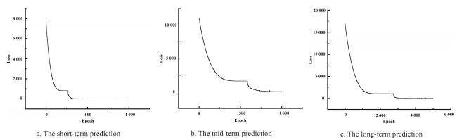
Fig. 4 Variation of loss with training epochs under different prediction horizons in tomato height prediction study |
From the Table 5 and Table 6, the PFE-RNN demonstrates limited advantages over the mono-modal RNN in short-term and medium-term predictions. However, it achieved significantly better performance in long-term predictions. This indicates that the PFE in the multi-modal model effectively captures essential characteristics of prolonged plant growth, thereby demonstrating greater reliability over extended timeframes. For instance, in the long-term setting (30-12), the PFE-RNN model with three layers and a hidden layer size of 20 achieves an MSE of 180.16 and a MAPE of 7.14%, whereas the mono-modal RNN shows an MSE of 1 140.67 and a MAPE of 17.18%. These results highlight the multi-modal model's substantial improvements in predictive accuracy in long-term forecasts. Additionally, a vertical comparison within the mono-modal model results reveals considerable fluctuations. For example, the mono-modal RNN with three layers and a hidden layer size of 20 reaches a high MAPE error of 22.76%, with substantial variations observed across other configurations as well. This indicates that predictions based on mono-modal input may be unstable and inaccurate.
The selected hyperparameter combination, which demonstrated better performance on the validation set, was further evaluated on the test set. The results are presented in Table 7. A short-term forecast with an error of ≤2% was considered accurate, a medium-term forecast with an error of ≤5% was considered accurate, and a long-term forecast with an error of ≤16% was considered accurate. The formula for calculating accuracy is provided in Equation (5) , and the results are summarized in Table 7.
Table 7 The optimal predictive performance of PFE-RNN in tomato height prediction study |
| Prediction scenario | Average accuracy/% | Last day accuracy/% | Average percentage error/% | Last day average percentage error/% | R 2 |
|---|---|---|---|---|---|
| Short-term prediction | 91.67 | 91.67 | 0.81 | 0.83 | 0.999 678 |
| Mid-term prediction | 88.54 | 87.50 | 2.66 | 3.11 | 0.991 119 |
| Long-term prediction | 70.37 | 66.67 | 14.05 | 16.63 | -0.041 393 |
The distribution of actual values and predicted values on the last day for the three predictions on the test set is shown in Fig. 5.
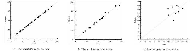
Fig. 5 Distribution of predicted values versus actual values for PFE-RNN prediction in tomato height values |
3.2 LSTM temporal prediction and model hyperparameter selection
Table 8 Parameters for LSTM operation in tomato height prediction |
| Network structure | Parameters |
|---|---|
| Input features | 34 |
| LSTM hidden size | 30 |
| LSTM layers | 2 |
| Learning rate | 0.001 |
| Loss function | MSELoss |
| Optimizer | Adam |
Similarly, Fig. 6 shows the variation of loss with training epochs under different prediction horizons in the tomato height prediction study. The loss curves demonstrate how the LSTM model adapts to varying temporal dependencies. The consistent decrease in loss across epochs indicates that the model effectively learns the complex relationships between input features and tomato height, validating the hyperparameter choices and the overall architecture design.
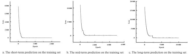
Fig. 6 Variation of loss with training epochs under different prediction horizons in tomato height prediction study |
Table 9 Results of multi-modal prediction using LSTM under different hyperparameters in tomato height prediction study |
| LSTM network layers | Hidden layer size | Prediction scenario | |||||
|---|---|---|---|---|---|---|---|
| Short-term prediction | Mmid-term prediction | Long-term prediction | |||||
| MSE | MAPE/% | MSE | MAPE/% | MSE | MAPE/% | ||
| 2 | 15 | 1.48 | 0.96 | 121.90 | 8.44 | 153.98 | 7.61 |
| 20 | 3.27 | 1.33 | 104.02 | 7.99 | 204.30 | 8.82 | |
| 25 | 0.57 | 0.88 | 88.01 | 6.63 | 254.83 | 9.67 | |
| 30 | 3.85 | 2.24 | 119.26 | 8.42 | 188.33 | 8.56 | |
| 3 | 15 | 0.21 | 0.54 | 81.72 | 7.60 | 547.96 | 15.03 |
| 20 | 1.56 | 1.44 | 105.02 | 8.89 | 286.87 | 10.56 | |
| 25 | 0.91 | 0.99 | 87.00 | 7.09 | 286.13 | 8.62 | |
| 30 | 0.34 | 0.73 | 98.91 | 7.16 | 172.19 | 6.54 | |
Table 10 Results of mono-modal prediction using LSTM under different hyperparameters in tomato height prediction study |
| LSTM network layers | Hidden layer size | Prediction scenario | |||||
|---|---|---|---|---|---|---|---|
| Short-term prediction | Mid-term prediction | Long-term prediction | |||||
| MSE | MAPE/% | MSE | MAPE/% | MSE | MAPE/% | ||
| 2 | 15 | 6.68 | 1.83 | 31.11 | 3.39 | 802.94 | 15.17 |
| 20 | 2.99 | 1.40 | 18.01 | 2.56 | 378.78 | 9.44 | |
| 25 | 6.59 | 2.22 | 39.56 | 4.25 | 486.95 | 11.55 | |
| 30 | 5.15 | 1.52 | 30.60 | 3.43 | 358.90 | 9.49 | |
| 3 | 15 | 3.79 | 1.37 | 37.67 | 3.79 | 870.38 | 15.67 |
| 20 | 3.89 | 1.39 | 21.53 | 2.84 | 507.24 | 10.95 | |
| 25 | 3.41 | 1.40 | 30.07 | 3.58 | 485.04 | 11.79 | |
| 30 | 7.01 | 1.74 | 153.36 | 7.81 | 385.27 | 8.66 | |
As demonstrated in Table 9 and Table 10, critical network parameters, including the number of layers and hidden layer dimensions, exerted a substantial influence on prediction accuracy, particularly in the PFE-LSTM model. For shorter input sequences (5-2), the PFE-LSTM configuration incorporating two layers with a hidden size of 25 demonstrated superior performance, achieving a MSE of 0.57 and a MAPE of 0.88%. However, when processing extended sequences (30-12), the model exhibited a marked degradation in performance, as evidenced by significantly elevated MSE and MAPE values (e.g., MSE = 286.87 with three layers and a hidden size of 20). This performance pattern suggests that increased parameter complexity or deeper network architectures may compromise predictive stability when handling longer temporal sequences. Based on comprehensive validation set evaluations, the optimal model configuration was selected and subsequently evaluated on the test set. The corresponding performance metrics are systematically presented in Table 11.
Table 11 Optimal predictive performance of PFE-LSTM model in tomato height prediction study |
| Prediction scenario | Average accuracy/% | Last day accuracy/% | Average percentage error/% | Last day average percentage error/% | R 2 |
|---|---|---|---|---|---|
| Short-term prediction | 97.92 | 97.92 | 0.40 | 0.38 | 0.999 901 |
| Mid-term prediction | 53.13 | 41.67 | 6.36 | 7.72 | 0.965 263 |
| Long-term prediction | 50.93 | 33.33 | 14.49 | 19.48 | -0.277 455 |
The distribution of actual values and predicted values on the last day for the three predictions on the test set is shown in Fig. 7.
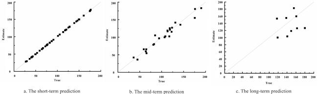
Fig. 7 Distribution of predicted values versus actual values for PFE-LSTM model |
3.3 Comparative analysis results with other methods
3.3.1 Performance evaluation of LLM
LLMs have emerged as a prominent approach for multimodal data processing. In this study, the identical image datasets and structured data were employed as input features for the advanced LLM architecture, specifically utilizing Zhipu Qingyan's GLM-4V-Plus model, to predict plant growth height. Given the inherent instability in the model's output generation, a rigorous manual filtering process was implemented to ensure the selection of the most reliable predictions.
The comparative analysis revealed that the LLM approach demonstrated moderate predictive accuracy for shorter sequence predictions (5-2 and 10-4 scenarios). However, the model exhibited significant limitations in processing extended temporal sequences (30-12 scenario), potentially attributable to challenges in effectively interpreting long-range dependencies within the input data. Consequently, these results were excluded from the final comparative analysis. The comparative performance metrics of the LLM approach are systematically presented in Fig. 8.
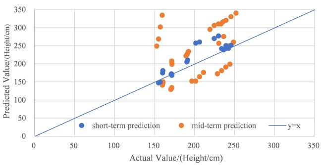
Fig. 8 Distribution of predicted values versus actual values for LLM prediction in tomato height |
3.3.2 Performance evaluation of Transformer-based model
Transformer-based models are another commonly used approach for processing multimodal and time-series data. In this study, a transformer-based model was implemented as a comparative baseline, employing identical images datasets and structured data as inputs features for plant growth height prediction. The experimental results revealed that the transformer outperformed the LLM approach in shorter sequence predictions (5-2 and 10-4 scenarios), demonstrating superior predictive accuracy. It similarly failed to capture the relationship between the input and plant height in the 30-12 scenario. This limitation is potentially attributable to two key factors of the increased task complexity and the longer input sequence. These findings suggest that the transformer struggles to effectively integrate temporal and spatial features for long-term predictions. The predictions of the transformer model are shown in Fig. 9, while the comparison results of the LLM, transformer, and LSTM models are presented in Table 12.
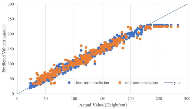
Fig. 9 Distribution of predicted values versus actual values for transformer prediction of tomato height |
Table 12 Comparison of results from different methods of tomato height prediction study |
| Model | Prediction scenario | MAPE/% | MSE | Last day MAPE/% |
|---|---|---|---|---|
| PFE-RNN | Short-term prediction | 0.81 | 0.56 | 0.83 |
| Mid-term prediction | 2.66 | 17.04 | 3.11 | |
| Long-term prediction | 14.05 | 651.35 | 16.63 | |
| PFE-LSTM | Short-term prediction | 0.40 | 0.12 | 0.38 |
| Mid-term prediction | 6.36 | 82.54 | 7.72 | |
| Long-term prediction | 14.49 | 696.22 | 19.48 | |
| Transformer | Short-term prediction | 6.72 | 74.71 | 6.33 |
| Mid-term prediction | 10.29 | 144.62 | 9.65 | |
| LLM | Short-term prediction | 8.00 | 588.26 | 7.90 |
| Mid-term prediction | 27.43 | 4 067.70 | 28.93 |
As shown in Table 12, the PFE model demonstrated superior predictive capabilities across all experimental configurations, outperforming both the LLM and the transformer model. Specifically, the PFE-RNN and PFE-LSTM models exhibited remarkable performance stability, achieving significantly lower MAPE and MSE values in both short-term (5-2) and medium-term (10-4) prediction scenarios. For instance, in the short-term prediction scenario, the PFE-RNN model achieved a MAPE of 0.81% and an MSE of 0.56, while the PFE-LSTM model achieved an even lower MAPE of 0.40% and an MSE of 0.12. In contrast, the transformer model achieved a MAPE of 6.72% and an MSE of 74.71, and the LLM performed even worse with a MAPE of 8.00% and an MSE of 588.26. In the medium-term prediction scenario, the PFE-RNN model maintained a MAPE of 2.66% and an MSE of 17.04, while the PFE-LSTM model achieved a MAPE of 6.36% and an MSE of 82.54. The transformer model, although better than the LLM, still underperformed with a MAPE of 10.29% and an MSE of 144.62, while the LLM struggled significantly with a MAPE of 27.43% and an MSE of 4 067.70. In the long-term prediction scenario (30-12), the PFE models continued to exhibit stable and reliable performance. The PFE-RNN model achieved a MAPE of 14.05% and an MSE of 651.35, while the PFE-LSTM model achieved a MAPE of 14.49% and an MSE of 696.22. Although the transformer model outperformed the LLM in this scenario, it still exhibited fundamental limitations, significantly higher than the PFE models. The LLM, on the other hand, demonstrated the least robust performance, highlighting its inability to effectively capture long-term temporal relationships.
This performance pattern suggests fundamental limitations in the LLM's ability to process and interpret complex temporal relationships in plant growth prediction tasks, despite rigorous manual filtering. The PFE models, particularly the PFE-RNN and PFE-LSTM, consistently outperformed both the transformer and LLM models across all prediction scenarios, demonstrating their robustness and accuracy in capturing the intricate relationships between input features and plant height.
4 Discussion
This study presents a Phenotypic Feature Extraction (PFE) model, which demonstrates significant advantages in predicting tomato growth height using multimodal data. In contrast to unimodal approaches, such as RNN and LSTM models that depend exclusively on either environmental data or images, the PFE model effectively integrates phenotypic and temporal features to construct a unified spatiotemporal representation, thereby significantly improving prediction accuracy.
In contrast to previous studies[23, 24] that primarily use remote sensing and large-scale data, this research leverages easily accessible RGB images and fine-grained environmental sensor data, combined with individualized plant monitoring, to capture more fine-grained crop phenotypic information. This approach addresses the limitations of remote sensing in handling detailed crop characteristics while offering greater applicability and operational simplicity. Aligning with the work of Lin et al.[25] on predicting lettuce fresh weight using RGB-D images, this study's multimodal integration further investigates the nonlinear interactions between plant growth and environment factors, thereby enabling more rubost and stable predictions under complex conditions.
Furthermore, the findings indicate that the PFE-LSTM model exhibits lower error variation in long-sequence prediction scenarios (e.g., 30-12), consistent with prior research that highlights the role of multimodal data fusion in mitigating overfitting. For instence, Tang et al.[30] pointed out that multimodal sensor fusion technology can obtain more reliable, informative, and accurate data by extracting and combining multimodal information. Compared to LLMs, the PFE model also demonstrates significant advantages in computational efficiency and interpretability, particularly for tasks involving longer input sequences. Its superior prediction accuracy further validates its potential for applications in precision agriculture.
Despite the promising results, there are some limitations in this study. For instance, it does not explore the applicability of the proposed model across different regions or latitudes. Future studies could expand to larger geographic areas and incorporate additional factors such as topography and climate variability to analyze the spatial dynamics of suitable sowing periods and growth patterns. Such efforts would enhance the generalizability and robustness of the findings.
Future work will focus on developing more granular crop growth models based on multimodal data, capturing dynamic growth changes by incorporating a wider range of multimodal inputs. Additionally, the model structure will be further refined through integration with established crop growth optimization models such as Agricultural Production Systems sIMulator (APSIM) or Decision Support System for Agrotechnology Transfer (DSSAT) to explore the applicability of the PFE model across different crop species, growth stages, and geographic regions. This approach aims to enhance the model's versatility and precision in addressing complex agricultural scenarios.
5 Conclusions
In this study, deep learning models were employed to predict tomato growth using multimodal data, encompassing environmental factors and plant images. By integrating phenotypic and temporal features, the research aimed to enhance prediction accuracy and analyze the interactions between plant and their environment.
The results showed that the PFE-RNN model achieved the best performance, with a MAPE of 0.81% in short-term (5-2) predictions and 2.66% in medium-term (10-4) predictions, demonstrating its effectiveness in capturing plant growth dynamics. The PFE framework proved particularly valuable by integrating spatial (image) and temporal (environmental) features, enabling accurate and stable predictions.
This study highlights the importance of selecting suitable model architectures and data scales for plant growth prediction. Future work should focus on expanding datasets and exploring advanced temporal models to further improve accuracy and generalization, thereby supporting precision agriculture through improved crop management and sustainability.


