欢迎您访问《智慧农业(中英文)》官方网站! English
信息处理与决策

基于改进VMD-LSTM的作物冠层温度动态预测模型

  • 王毓玺 1 ,
  • 黄铝文 , 1, 2 ,
  • 段小琳 1
展开
  • 1. 西北农林科技大学 信息工程学院,陕西杨凌 712100,中国
  • 2. 农业农村部农业物联网重点实验室,陕西杨凌 712100,中国
黄铝文,博士,副教授,研究方向为生物图像处理。E-mail:

王毓玺,硕士研究生,研究方向为生物图像处理。E-mail:

收稿日期: 2025-02-20

  网络出版日期: 2025-05-22

基金资助

国家重点研发计划项目(2020YFD1100601)

Dynamic Prediction Model of Crop Canopy Temperature Based on VMD-LSTM

  • WANG Yuxi 1 ,
  • HUANG Lyuwen , 1, 2 ,
  • DUAN Xiaolin 1
Expand
  • 1. College of Information and Engineering, Northwest A&F University, Yangling 712100, China
  • 2. Key Laboratory of Agricultural Internet of Things, Ministry of Agriculture and Rural Affairs, Yangling 712100, China
HUANG Lyuwen. E-mail:

WANG Yuxi. E-mail:

Received date: 2025-02-20

  Online published: 2025-05-22

Supported by

National Key R&D Program of China(2020YFD1100601)

Copyright

copyright©2025 by the authors

摘要

【目的/意义】 准确预测作物冠层温度,有助于综合衡量作物生长状况、指导农业生产。本研究以猕猴桃和葡萄为研究对象,解决作物冠层温度预测的准确性问题。 【方法】 构建一种基于长短期记忆(Long Short-Term Memory, LSTM)网络、变分模态分解(Variational Mode Decomposition, VMD)和雾凇优化算法(Rime Ice Morphology-based Optimization Algorithm, RIME)的作物冠层温度动态预测模型RIME-VMD-RIME-LSTM(即RIME2-VMD-LSTM)。首先,通过悬挂于滑索上的园区巡检机器人采集作物冠层温度数据。其次,通过多组预测试验的性能表现,选定VMD-LSTM作为基模型,同时为减小VMD不同频率分量之间交叉干扰,运用K-means聚类算法对各分量样本熵进行聚类,重构为新分量。最后,利用RIME优化算法对VMD和LSTM的参数进行优化,提升模型的预测精度。 【结果和讨论】 本模型在模拟不同噪声环境下的均方根误差(Root Mean Square Error, RMSE)和平均绝对误差(Mean Absolute Error, MAE)均小于对比模型,分别为0.360 1和0.254 3 ℃,且R2高达0.994 7。 【结论】 本研究模型为动态预测作物冠层温度提供了可行的方法,并为园区作物生长状况提供数据支持。

本文引用格式

王毓玺 , 黄铝文 , 段小琳 . 基于改进VMD-LSTM的作物冠层温度动态预测模型[J]. 智慧农业, 2025 , 7(3) : 143 -159 . DOI: 10.12133/j.smartag.SA202502015

Abstract

[Objective] Accurate prediction of crop canopy temperature is essential for comprehensively assessing crop growth status and guiding agricultural production. This study focuses on kiwifruit and grapes to address the challenges in accurately predicting crop canopy temperature. [Methods] A dynamic prediction model for crop canopy temperature was developed based on Long Short-Term Memory (LSTM), Variational Mode Decomposition (VMD), and the Rime Ice Morphology-based Optimization Algorithm (RIME) optimization algorithm, named RIME-VMD-RIME-LSTM (RIME2-VMD-LSTM). Firstly, crop canopy temperature data were collected by an inspection robot suspended on a cableway. Secondly, through the performance of multiple pre-test experiments, VMD-LSTM was selected as the base model. To reduce cross-interference between different frequency components of VMD, the K-means clustering algorithm was applied to cluster the sample entropy of each component, reconstructing them into new components. Finally, the RIME optimization algorithm was utilized to optimize the parameters of VMD and LSTM, enhancing the model's prediction accuracy. [Results and Discussions] The experimental results demonstrated that the proposed model achieved lower Root Mean Square Error (RMSE) and Mean Absolute Error (MAE) (0.360 1 and 0.254 3 °C, respectively) in modeling different noise environments than the comparator model. Furthermore, the R2 value reached a maximum of 0.994 7. [Conclusions] This model provides a feasible method for dynamically predicting crop canopy temperature and offers data support for assessing crop growth status in agricultural parks.

0 Introduction

In agricultural production, canopy temperature is a crucial research indicator that affects crop growth, disease and insect control, and water and fertiliser management[1, 2]. One of the key management techniques to maximise crop growth and development is crop canopy temperature prediction, which may also yield data to assist crop growth. Researchers mostly used methods based on physical models and empirical equations to predict canopy temperature. In a greenhouse environment, Jeon et al.[3] developed a plant model to calculate canopy temperature by using Leaf Area Index (LAI), crop light, transpiration, canopy temperature, and heat flux, and proved the reliability of the model by comparing it with the field measurements. Shao et al.[4] proposed a periodic coefficient probabilistic model for predicting canopy temperature using weather variables, which can capture the nonlinear relationship between daily changes in canopy temperature and weather variables based on the coefficients of time variations during the day. Although these methods show potential in predicting canopy temperature, they have high requirements for the accuracy and stability of environmental parameters and are somewhat limited in their application scope. Therefore, developing a model capable of achieving real-time and accurate prediction of canopy temperature is of great significance for the management of the entire crop growth cycle.
In recent years, machine learning and deep learning have been widely employed in the modeling and prediction of crop growth and environmental information. Yang et al.[5] employed the Random Forest (RF) model to predict the canopy temperature of oilseed rape in China, and the model's effectiveness was validated by simulating the upper and lower bounds of canopy temperature using two distinct datasets. Andrade et al.[6] applied Artificial Neural Networks (ANNs) to predict the canopy temperature of corn in Texas, and the Root Mean Square Error (RMSE) values for the two sets of experiments ranged from 1.04 to 2.49°C and 2.14 to 2.77°C, respectively. Kondo et al.[7] developed a novel neural network model for predicting canopy temperature using only meteorological data, the model exhibited high accuracy, capturing 94.8% of the observed data within the canopy temperature range from -4 to 2°C. Yoshimoto et al.[8] predicted heat-induced glume sterility in rice across different climatic regions by integrating the MiNCERnet monitoring network (a multi-site system with micrometeorological sensors for rice canopy environments) with the IM2PACT model (a heat-balance model to estimate panicle temperature of rice), enhanced the accuracy of predicting climate change impacts and contributed to developing effective adaptation strategies for rice cultivation. Banerjee et al.[9] proposed a machine learning method to predict net crop surface radiation. Global solar radiation and canopy temperature were used as input. Results showed that gradient boosted regression and ridge regression performed better than other machine learning methods. Although the above methods achieved great performance, they struggled with complex environmental changes and long-term dependencies. Their generalization also remained limited.
To address these challenges, researchers have employed Long Short-Term Memory (LSTM) networks for crop growth and environmental prediction. LSTM excels in sequence modeling by capturing nonlinear temporal dynamics and selectively retaining critical information, overcoming long-term dependency issues in time-series data[10]. Its ability to model seasonal variations and climate impacts enhances prediction accuracy and robustness. Tian et al.[11] used a bi-directional LSTM (Bi-LSTM) model to predict wheat yield. The model combined remote sensing and meteorological data, achieved the highest accuracy at two time steps (R 2=0.83, RMSE=357.77 kg/ha), outperformed the Back Propagation Neural Network (BPNN) and Support Vector Machine (SVM). The model also adapted well to different climatic conditions. Kiran Kumar et al.[12] developed optimized LSTM and Bi-LSTM models to predict wheat, peanut, and barley yields in India. Hyper-parameter optimization was used in model training. The results showed that Bi-LSTM performed better than traditional machine learning models. For wheat and peanut, the prediction errors were reduced by 39% and 13% respectively. Zhang et al.[13] proposed a Principal Component Selection - Long Short-Term Memory (​PCS-LSTM) model that enhanced multi-site temperature prediction by integrating periodicity and the social pooling mechanism of neighboring sites. Results illustrated that the Mean Absolute Error (MAE) reduced by 0.109°C in the 24-hour prediction. Pang et al.[14] developed a LSTM model integrated with a Particle Swarm Optimization(PSO) algorithm to predict global average temperature. Compared with BP, PSO-BP, and standard LSTM models, PSO-LSTM achieved lower error metrics, with a Mean Squared Error (MSE) of 0.280 7°C and a Mean Absolute Percentage Error (MAPE) of 0.004 5. The model improved prediction accuracy and provided a novel method for temperature forecasting.
In this study, a suspended inspection robot platform to collect canopy temperature data form kiwifruit and grape orchards was utilized. A LSTM neural network was subsequently applied to analyze the data, culminating in the development of the Rime Ice Morphology-based Optimization Algorithm-Variational Mode Decomposition-Rime Ice Morphology-based Optimization Algorithm-Long Short-Term Memory (RIME2-VMD-LSTM) for crop canopy temperature prediction. The model's performance was comprehensively evaluated using multiple assessment metrics. By integrating advanced agricultural robotics with computational intelligence, this work provides a technical foundation for precision temperature monitoring in orchard crops, thereby supporting intelligent agricultural production.

1 Materials and methods

1.1 Data collection

Crop canopy temperature data was collected using a sliding contact-powered zipline intelligent inspection robot. To better adapt to the outdoor environment, complete operational tasks efficiently, and facilitate later maintenance and upgrading, the intelligent inspection robot was designed in a modular and divided into three major parts, as shown in Fig.1a. The inspection platform consists of tower base, servo motor, reducer, and traction and load-bearing cables. The vehicle body had miniature weather sensors, temperature recorders, and other data acquisition equipment. The traction wire was fixed to the robot body, and the servo motor drove it back to move the vehicle body. The control cabin was equipped with an industrial control computer, motor drives, and 220 V alternating current (AC) power and Ethernet ports. A dual-end low-voltage sliding contact system was adopted to optimize the cable-based power supply method. The 220 V AC mains power was routed to the control cabin and split into two circuits: One directly powered the control box equipment, while the other passed through an adjustable switching power supply(0~70 V), converted it to a 40 V low-voltage safety direct current (DC). This DC power was transmitted via a conductive load-bearing cable to supply the onboard robotic systems. Data transmission was facilitated via a wireless bridge and Gigabit optical fiber. The robotic platform also integrated compact weather sensors, which communicated via RS485 protocol and were adapted to Ethernet through signal conversion. Additionally, it carries a camera, wireless bridge receiver, and connected to a switch to receive control commands from the server, as shown in Fig.1b.
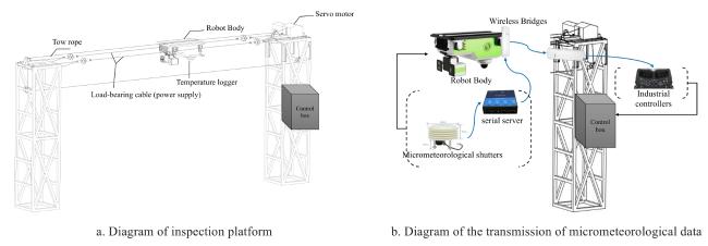
Fig. 1 Composition diagram of agricultural inspection robot system
The study was conducted at the Yangling Comprehensive Agricultural Experiment and Demonstration Station (34°18′4.24″N, 107°58′10.26″E), in Wuquan town of Northwest Agriculture and Forestry University, located in Yangling Agricultural Hi-Tech Industrial Demonstration Zone, Shaanxi province. This site shares climatic conditions with major kiwifruit (Zhouzhi County) and grape (Huyi District) production areas in Shaanxi. The experimental area was the adjacent kiwifruit and grape plots in the demonstration station (as shown in Fig. 2). Based on the demonstration station layout, a data collection area was delineated. Temperatures of crop canopy were dynamically recorded using an inspection robot mounted on a 3 m-high, 300 m-long rail platform. Infrared temperature loggers (specifications are listed in Table 1) were installed beneath the robot, either near or within the leaf clusters, to directly capture infrared radiation emitted from the crop canopy. To minimize environmental interference, the sensors were equipped with shielding covers to reduce the effects of direct sunlight and air flow.
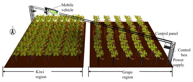
Fig. 2 Diagram of plantation area plotted by Unity software
Table 1 Parameters of temperature recorder of data preprocessing study
Parameter Specification
Measurement range -20~80 ℃
Measurement accuracy ±0.5 ℃
Response time ≤1 s
Operating environment -40~85 ℃, Humidity ≤95%RH
Data storage frequency Every 10 minutes
To prevent rainfall from affecting the logger, a conical plastic cover was placed over it. This protection allowed the sensors to maintain direct contact with the air while shielding them from rain. The data storage frequency of the equipment was once every 10 minutes. For reducing the time scale difference between canopy temperature, atmospheric meteorological data, and micrometeorological data, the three types of data sheets were fused to obtain meteorological data sheets with the same time scale. The 10-minute span data from April 2023 to August 2023 were selected to construct the environmental multivariate dataset for kiwifruit and grape canopies in the experimental orchard, with a dataset size of 22 320 entries.

1.2 VMD-LTSM

1.2.1 LTSM

LSTM networks feature a unique hidden layer unit structure. In this structure, neuron input includes not only current moment data but also previous moment state input. This design endows models with robust contextual memory capabilities, addressing issues of long-term dependency, gradient vanishing, and gradient explosion in Recurrent Neural Networks (RNNs). Therefore, LSTM networks was selected to construct canopy temperature prediction model.
LSTM networks consist of three gates: forget gate, input gate and output gate[15]. Each hidden layer unit within LSTM comprises three gates: input gate ( i), output gate ( o), forgetting gate ( f  ), along with a memory cell that retains long-term data characteristics within the loop structure. Forget gate controls retention or discarding of information from previous moment memory cells with a certain probability. Input gate determines new information to be stored in current cell state, while output gate regulates information output from current cell. These "gates" selectively control flow of information as needed.

1.2.2 VMD time series data decomposition and reconstruction

Since both the crop canopy temperature data collection environment and the prediction model application scenario are outdoor orchard environments, the data are susceptible to noise interference. To address this, the VMD method was used to decompose the data and reduce the noise before inputting it into the LSTM network for prediction[16, 17]. The VMD decomposition method was developed on the basis of Empirical Mode Decomposition (EMD), which was a completely non-recursive decomposition algorithm that can decompose complex data into simple data with different center frequencies[18]. Each component generated by the decomposition was the intrinsic mode function (IMF) of the original data, and the superposition of all IMFs reconstructeds the original data. VMD adaptively achieved signal frequency domain segmentation and effective component separation. Compared with the other signal decomposition methods, it exhibited superior denoising and modal aliasing suppression capabilities, meeting the requirements for decomposition and noise reduction of canopy temperature time series data[19].
Assuming that the initial signal was decomposed into K IMF, the analytic signal was first constructed for each IMF using the Hilbert transform, and the one-sided spectrum was computed. Next, the spectrum was shifted to its corresponding baseband based on the displacement property of the Fourier transform. Finally, the bandwidth of each IMF was estimated using the Gradient-squared L 2, and the sum of the spectral widths of all the IMFs was minimized, which transformed it into an unconstrained variational problem as in Equation (1) before solving the individual modal components.
m i n { u k } , { ω k } k = 1 K t δ ( t ) + j π t * u k ( t ) e - j ω k t 2 2 ,     s . t .   k u k = f
Where, ω k is the set of center frequencies of each IMF; K is the number of decomposed IMF components; t is time partial derivative; δ ( t ) is Dirac function; u k ( t ) is the k-th IMF; j is Imaginary unit; * is convolution operation; k is time variable; ( δ ( t ) + j / π t ) * u k ( t ) is Hilbert transform.
The Lagrange multiplier λ ( t ) as well as the quadratic penalty factor α are introduced to turn Equation (1) into an unconstrained variational problem, and the augmented Lagrange expression is constructed as Equation (2). And the Alternate Direction Method of Multipliers (ADMM) operator is used to solve the problem.
L u k , ω k , λ = α k = 1 K t δ ( t ) + j π t * u k ( t ) e - j ω k t 2 2              + f ( t ) - k = 1 K u k ( t ) 2 2 + λ ( t ) , f ( t ) - k u k ( t )
Where, f is initial signal; · is inner product arithmetic; λ ( t ) is Lagrange multiplier.
After updating each mode and its center frequency in the frequency domain, the signals were transformed into the time domain. The IMFs and their center frequencies were obtained through the VMD. In this study, VMD was applied to decompose the canopy temperature data of kiwifruit and grape separately. Each original temperature series was decomposed into ten IMFs: {IMF1, IMF2, …, IMF10}. As shown in Fig. 3, IMF1 captured the long-term trend of the canopy temperature. The remaining components fluctuated around zero and showed high-frequency volatility.
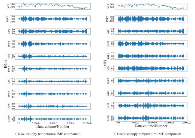
Fig. 3 Results of VMD decomposition
To reduce the cross-interference among frequency components and enhance the independence of each mode, the K-means clustering algorithm was applied to the sample entropy of each component. The components were then reconstructed into new groups. Sample entropy measures the complexity and irregularity of time series signals. K-means is a partition-based clustering algorithm, its goal is to maximize similarity within clusters and minimize similarity between clusters[20]. The reconstruction process (shown in Fig. 4) involved: 1) calculating IMF sample entropy via sample_entropy(); 2) clustering results using K-means_cluster(); 3) summing co-clustered modes and sorting by descending sample entropy.
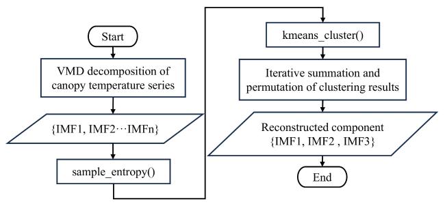
Fig. 4 Flowchart of reconstruction with K-means
The K-means algorithm first requires specifying the constant K, which defined the number of clusters. Then, K samples were randomly selected as the initial centroids. The distance between each data point and each centroid was calculated, and each point is assigned to the nearest cluster. After assignment, the centroid of each cluster was updated by computing the mean of all points in that cluster. These two steps-assignment and centroid update-are repeated until the centroids converge or a preset number of iterations was reached. Once convergence was achieved, the final cluster labels and centroids was determined. Using this process, the reconstructed IMF* components were obtained, as shown in Fig. 5.
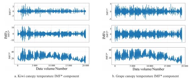
Fig. 5 Results of reconstruction with K-means

1.3 RIME2-VMD-LSTM model construction

To enhance the temporal features of canopy temperature data, reduce noise, and improve prediction accuracy for kiwifruit and grapes, a VMD-LSTM model was used as the base prediction framework. The time-series canopy temperature data served as the model input. To further reduce prediction error and improve performance, the RIME optimization algorithm was applied to optimize both LSTM and VMD parameters. This led to the construction of the RIME2-VDM-LSTM prediction model. The decomposed components {IMF1, IMF2, …, IMFn} were clustered and reconstructed into new components {IMF1*, IMF2*, IMF3*}. These were used as inputs to the optimized LSTM model for training and prediction. The outputs were then linearly superimposed and inverse normalized. The overall framework of the model is depicted in Fig. 6.
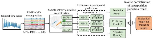
Fig. 6 Framework of RIME2-VMD-LSTM model

1.3.1 VMD-RIME-LSTM

To optimize the VMD-LSTM model and improve canopy temperature prediction accuracy, this study determined the optimal parameters of each reconstructed IMF* component before LSTM input. Among five classical optimization algorithms (e.g., subsection 2.3.2), the RIME algorithm a 2023 metaheuristic inspired by freezing fog physics[21] was selected for LSTM parameter tuning. RIME simulates rime growth mechanisms by modeling fog droplets as intelligent agents interacting with environmental factors (e.g., temperature, wind speed), establishing soft-rime search and hard-rime puncture strategies. The RIME algorithm comprises four steps:
1) Fog population initialisation. Initialize a frozen population R with n agents, each containing d fog particles.
2) Soft freezing search strategy. Leverages the randomness of soft-rime particles in breezes to enhance early-stage exploration and avoid local optima.
3) Hard freezing puncture mechanism. Inspired by wind-driven aligned growth, enables inter-particle information exchange to accelerate convergence.
4) Positive greedy selection mechanism. Retains updated solutions with better fitness values to improve global search efficiency and population diversity.
The flowchart of the VMD-RIME-LSTM model is shown in Fig. 7 and the flowchart of the RIME optimization of the LSTM parameters is shown in Fig. 8.
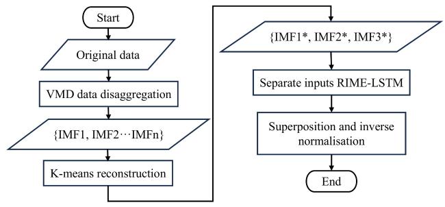
Fig. 7 Flowchart of VMD-RIME-LSTM model
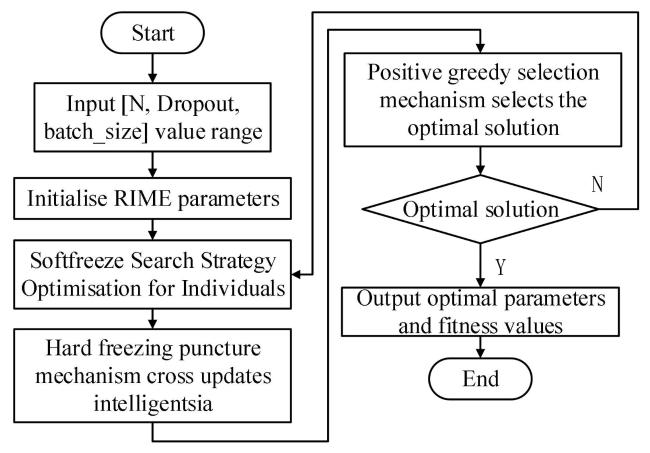
Fig. 8 Flowchart of optimizing LSTM parameters with RIME algorithm

1.3.2 RIME-VMD

In order to avoid the randomness and irrationality of artificially set VMD parameters in the calculation process, the RIME algorithm was adopted to select the maximum value of the sample entropy and sought the optimization of the penalty factor α and the number of modes K in the VMD. Therefore, in the VMD-RIME-LSTM prediction model, the original VMD decomposition method was replaced with the RIME-VMD optimal decomposition approach to construct the RIME-VME-RIME-LSTM model (RIME2-VMD-LSTM), which extracted the main features of the canopy temperature data and maximize the information retention. The RIME-optimized VMD process was similar to RIME-optimized LSTM. In RIME-VMD, optimization was performed for the penalty factor α and the number of modes K in VMD.

2 Results and analysis

2.1 Evaluation indicators and environmental settings

In order to fully assess the performance of the prediction model, RMSE[22], MSE, Coefficient of Determination (R-Squared, R 2), and MAE were used to evaluate the model. Among them, RMSE describes the deviation between the real value and the predicted value. MSE reflects the error of the predicted value, and MAE indicates the degree of dispersion of the prediction error. Combining each index to evaluate the precision and accuracy, the smaller the value, the smaller the error between the predicted value and the true value, indicating the better performance of the model, and the closer the coefficient of determination R 2 is to 1, the better the model fit.
The construction and improvement of the prediction model was based on the TensorFlow2.11.0 and Keras2.11.0 frameworks, and the training and testing of the model was carried out under the Windows system. The kiwifruit and grape canopy temperature data were taken out separately to construct the dataset for the prediction test in this paper, and the training set, validation set and testing set were divided according to 3:1:1.

2.2 Data smoothing analysis

In order to construct a dependable canopy temperature prediction model, it was essential to guarantee that the canopy temperature time series data complied with the smoothness assumption. Smoothness tests can be broadly classified into two categories: subjective and objective[23].In light of the inherent subjectivity of the subjective test method and its potential impact on the reliability of test outcomes, the ADF test, a representative objective test method was emploied, to conduct a smoothness assessment of the canopy temperature data.
The ADF test is to determine whether a unit root exists in the series by constructing a regression model such as Equation (3), which includes a first-order difference as well as a possible lag term, and the root of the equation is called a unit root if β is one. If the series is smooth, there is no unit root; otherwise, there is a unit root.
Δ y t = α + β y t - 1 + γ 1 Δ y t - 1 + γ 2 Δ y t - 2 + + γ p Δ y t - p + ε t
Where, Δ y t is time series with first-order differences; α is intercept; β is factors; γ i is coefficients of lag terms; ε t is error term.
In the ADF test, H 0 is assumed to be the existence of a unit root, and if the value of the significance test statistic T is found to be less than three confidence levels of 1%, 5% and 10%, then the original hypothesis H 0 is rejected with 99%, 95% and 90% certainty. Meanwhile, in hypothesis testing, it is also possible to determine whether there is enough evidence to reject the original hypothesis by whether the p is less than the significance levels of 0.05 and 0.01. When the p is less than 0.05, the unit root hypothesis is rejected, indicating that the data are smooth, if the p is greater than 0.05, the original hypothesis cannot be rejected and the data are not smooth, at which point it is necessary to differentiate the data or other treatments in order to achieve the smoothness requirements.
As outlined in Table 2, the Inspection results T of kiwifruit and grape canopy temperature are much smaller than the acceptance domain of the original hypothesis of the existence of a unit root, and at the same time p is much smaller than 0.01, so the original hypothesis of H 0 is rejected, and the data do not have a unit root, then the data are smooth. At the same time, it can be visualized from Fig. 9 that the trend of canopy temperature data of the 2 crops is generally smooth. In conclusion, through the smoothness test, it is proved that the canopy temperature data of kiwifruit and grape collected in this paper are significantly smooth data, which ensures that the data can meet the basic premise of predictive modelling.
Table 2 Results of ADF tested of data preprocessing study
Inspection parameters T  Inspection results P 1% Threshold 5% Threshold 10% Threshold
Kiwi canopy temperature -14.401 0.000 0 -3.960 -3.410 -3.120
Grape canopy temperature -11.700 0.000 0 -3.430 -2.860 -2.570
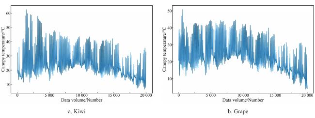
Fig. 9 Tendency of canopy temperature

2.3 Comparative experiments

2.3.1 VMD-LSTM base model

In order to verify the performance of the VMD-LSTM-based model, the results of the prediction and evaluation indexes of the LSTM model combined with different decomposition methods were compared. The LSTM conventional parameters were fixed by varying the number of neurons and the input sequence length (L in), where the number of neurons   { 50 ,   100 ,   150 ,   200 ,   250 } and L in   { 8 ,   16 ,   32 ,   64 }. The VMD-LSTM was combined with a single LSTM model, LSTM with EMD and complete Ensemble Empirical Mode Decomposition with Adaptive Noise (CEEMD), respectively. Complete Ensemble Empirical Mode Decomposition with Adaptive Noise (CEEMDAN)[24], Symmetric Geometric Mode Decomposition (SGMD), Time-Variant Filtered Empirical Mode Decomposition (TVF-EMED)[25] four decomposition algorithms of the combined prediction models were tested for comparison.
In the LSTM model training process, MSE was chosen as the loss function, MAE was used as the evaluation index, ReLU function was used as the activation function, and the adaptive estimation (Adam) optimizer was used for training, with the settings of epoch as 300, batch_size as 64, and learning_rate as 0.001, and the settings of Dropout as 0.1 were used for preventing overfitting. Dropout was set to 0.1. The decomposition algorithm parameters were set with default values. Each model was trained for 5 rounds and the model that predicted the validation set best was used to predict the test set. The kiwifruit and grape canopy temperature data were input into the models, and the test results with the best results were centered on when L in = 8 and L in = 16. Therefore, some of the prediction results are shown separately, as shown in Table 3 and Table 4.
Table 3 Prediction results of decomposition combination models with L in=8 of model forecasting study
Number of neurons/cell LSTM EMD-LSTM CEEMDAN-LSTM
MSE/℃ MAE/℃ MSE/℃ MAE/℃ MSE/℃ MAE/℃
50 0.479 0 0.535 0 0.215 0 0.303 5 0.216 5 0.280 5
100 0.456 5 0.473 0 0.148 0 0.278 0 0.329 0 0.348 0
150 0.909 5 0.786 5 0.188 5 0.304 0 0.169 5 0.272 0
200 0.327 0 0.389 0 0.249 5 0.310 5 0.215 5 0.302 5
250 0.405 5 0.447 5 0.233 0 0.326 5 0.289 5 0.337 0
Number of neurons/cell VMD-LSTM SGMD-LSTM TVF-EMD-LSTM
MSE/℃ MAE/℃ MSE/℃ MAE/℃ MSE/℃ MAE/℃
50 0.101 5 0.192 5 0.185 0 0.262 5 0.178 5 0.242 5
100 0.095 0 0.195 0 0.464 0 0.380 0 0.186 5 0.261 5
150 0.100 5 0.203 0 0.675 5 0.432 5 0.175 0 0.252 5
200 0.127 0 0.213 0 0.409 5 0.398 0 0.205 0 0.299 0
250 0.114 5 0.225 0 0.261 5 0.335 0 0.209 5 0.299 5

Note:Bold values in the table indicate the best performance for each category. Reported MSE and MAE values represent the mean results across both kiwifruit and grape canopy temperature datasets.

Table 4 Prediction results of decomposition combination models with L in=16 of model forecasting study
Number of neurons/cell LSTM EMD-LSTM CEEMDAN-LSTM
MSE/℃ MAE/℃ MSE/℃ MAE/℃ MSE/℃ MAE/℃
50 0.563 0 0.548 5 0.336 5 0.402 5 0.318 0 0.325 0
100 0.414 0 0.427 5 0.270 0 0.368 5 0.487 0 0.481 0
150 0.568 0 0.529 0 0.481 0 0.495 5 0.367 0 0.427 5
200 0.323 5 0.405 5 0.380 5 0.477 0 0.421 0 0.425 0
250 0.502 0 0.477 5 0.601 5 0.510 5 0.380 0 0.413 0
Number of neurons/cell VMD-LSTM SGMD-LSTM TVF-EMD-LSTM
MSE/℃ MAE/℃ MSE/℃ MAE/℃ MSE/℃ MAE/℃
50 0.273 5 0.325 5 0.282 5 0.369 5 0.416 5 0.415 5
100 0.282 0 0.390 5 0.437 0 0.475 5 0.348 0 0.440 5
150 0.257 0 0.320 0 0.930 5 0.604 0 0.273 5 0.370 0
200 0.250 0 0.326 5 0.713 5 0.543 5 0.267 0 0.357 0
250 0.278 0 0.325 0 0.662 5 0.524 5 0.249 0 0.315 5

Note:Bold values in the table indicate the best performance for each category. Reported MSE and MAE values represent the mean results across both kiwifruit and grape canopy temperature datasets.

From the results in Table 3, it can be seen that when L in=8 and the set of neuron numbers is { 50 ,   100 ,   150 ,   200 ,   250 }, the MSE and MAE values of VMD-LSTM are the lowest among the 6 models, and the average MSE of this model is 0.107 7°C and the average MAE is 0.205 7°C. Furthermore, in Table 4, when L in is 16, most of the minimum values of MSE and MAE among the six models appeared in VMD-LSTM, and by calculating the mean values of the evaluation indexes separately. It can be seen that the VMD-LSTM model has an average MSE=0.268 1°C and an average MAE=0.337 5°C, which are the lowest among the six models. The rest of the models are ranked in order of their composite indicators as TVF-EMD-LSTM, EMD-LSTM, CEEMDAN-LSTM, and SGMD-LSTM.
Moreover, the addition of five decomposition algorithms to the LSTM model decreases the MSE and MAE values to some extent compared to the single LSTM. Among them, VMD-LSTM decreased the most, when L in = 8, MSE and MAE decreased by 79.11% and 60.91%, respectively; when L in = 16, they decreased by 43.45% and 29.33%, respectively. SGMD-LSTM decreased the least, when L in = 8, MSE and MAE decreased by 22.58% and 31.28%, respectively; when L in = 16, MSE and MAE increased by 27.65% and 5.40%.
In order to further judge a more stable combined prediction model, under L i n { 8,16 } and the set of neuron numbers is { 50 ,   100 ,   150 ,   200 ,   250 }, the average degree of rise of MSE and MAE predicted by the model for the next 10 minutes to 1 hour is used as a judgment indicator for choosing the decomposition algorithm, and the experimental results are shown in Fig. 10. It is seen that in different data sets and different input lengths, the MSE and MAE of LSTM rise to the greatest extent, with an average rise of 4.255 1 and 1.009 5°C, respectively, and the VMD-LSTM indicator rises to the smallest extent on average, with the 2 indicators rising to an average of 1.793 9 and 0.592 5°C, respectively. In summary, the VMD-LSTM-based model proposed can reduce the MSE and MAE values predicted by a single LSTM model on canopy temperature time-series data, improve the model's interpretability, performance, and generalization ability, and apply to multi-step prediction with more stability relative to other decomposition algorithms.
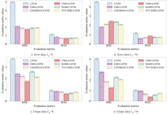
Fig. 10 Comparison chart of the average crease in evaluation metrics of model performance comparison study

2.3.2 RIME-LSTM optimization

To verify the effectiveness of RIME optimization of LSTM parameters, the VMD-RIME-LSTM model was compared with four optimization algorithms, namely the classical Particle Swarm Optimization (PSO), Sparrow Search Algorithm (SSA), Grey Wolf Optimizer (GWO) and Snow Ablation Optimizer (SAO). The kiwifruit and grape canopy temperatures were predicted for the next 1~3 hours, respectively, and the evaluation indexes RMSE and MAE were combined to assess the prediction effect of RIME after optimizing the LSTM parameters. The comparison model's key parameters were configured as follows: the optimization algorithm used a population size of 10, a maximum of 20 iterations, and 5 epochs; all other settings remained at their defaults. Search LSTM parameter range: number of neurons [1, 500], Dropout [0.001, 0.99], batch size [1, 300], epoch is 50.
The results of the predictive analysis are presented in Table 5. For kiwifruit canopy temperature data, the VMD-RIME-LSTM algorithm exhibits the lowest two metrics among the five optimization algorithms in predicting the next one-hour interval (RMSE=1.465 8°C, MAE=0.900 7 °C) and the subsequent two-hour interval (RMSE=2.873 9 °C, MAE=1.732 1 °C), while VMD-SSA-LSTM has the lowest RMSE and MAE values for predicting the next three-hour (RMSE=4.170 3 °C, MAE=2.502 7 °C). Combination the three different prediction lengths revealed that VMD-RIME-LSTM had the lowest mean RMSE and MAE values of 2.845 3 °C and 1.718 5 °C, respectively. In the case of grape canopy temperature data, the VMD-SAO-LSTM model exhibited the lowest RMSE and MAE values when predicting one hour into the future (RMSE=1.357 5 °C, MAE=0.876 6 °C). Furthermore, the VMD-SAO-LSTM model demonstrated the smallest RMSE values of the compared algorithms when predicting two and three hours into the future. The RMSE is lowest for VMD-RIME-LSTM (2.564 9 °C, 3.632 2 °C), while the MAE is lowest for VMD-RIME-LSTM (1.731 0 °C, 2.459 3 °C, respectively). Furthermore, the mean values of the three different prediction lengths also demonstrate the same results.
Table 5 Predicted results with different optimization algorithms of model forecasting study
Temp comparison models Next 1 hour Next 2 hours Next 3 hours Average
RMSE/℃ MAE/℃ RMSE/℃ MAE/℃ RMSE/℃ MAE/℃ RMSE/℃ MAE/℃
Kiwi canopy VMD-PSO-LSTM 1.498 0 0.943 8 2.958 7 1.818 0 4.251 3 2.604 3 2.902 7 1.788 7
VMD-SSA-LSTM 1.478 2 0.903 2 2.912 4 1.756 9 4.170 3 2.502 7 2.853 6 1.720 9
VMD-GWO-LSTM 1.481 3 0.915 8 2.897 2 2.302 2 4.186 4 2.549 6 2.855 0 1.922 5
VMD-SAO-LSTM 1.504 5 0.919 1 3.041 4 1.850 3 4.397 6 2.680 5 2.981 2 1.816 6
VMD-RIME-LSTM 1.465 8 0.900 7 2.873 9 1.732 1 4.196 3 2.522 8 2.845 3 1.718 5
Grapes canopy VMD-PSO-LSTM 1.371 2 0.882 4 2.620 0 1.770 5 3.685 6 2.581 5 2.558 9 1.744 8
VMD-SSA-LSTM 1.401 1 0.879 7 2.580 0 1.774 3 3.667 4 2.570 0 2.549 5 1.741 3
VMD-GWO-LSTM 1.418 7 0.902 8 2.664 6 1.756 5 3.744 4 2.514 0 2.609 2 1.724 4
VMD-SAO-LSTM 1.357 5 0.876 6 2.564 9 1.733 8 3.632 2 2.526 8 2.518 2 1.712 4
VMD-RIME-LSTM 1.378 6 0.897 3 2.611 8 1.731 0 3.635 7 2.459 3 2.542 0 1.695 9

Note:Bold values in the table indicate the best performance for each category. Reported RMSE and MAE values represent the mean results across both kiwifruit and grape canopy temperature datasets.

The average values of RMSE and MAE of the 5 methods on 2 datasets were further calculated, and it could be concluded that the RMSE of VMD-RIME-LSTM was lower than the first 4 models by 1.36%, 0.29%, 1.41%, 2.04%, and the MAE was lower than the first 4 models by 3.37%, 1.38%, 6.38%, and 3.25%, respectively. It is noted that all the above five optimization models perform well for multi-step prediction of the data in this paper, with VMD-RIME-LSTM giving the best overall performance for canopy temperature prediction for the two datasets at three different lengths of time.

2.3.3 RIME-VMD optimization

In order to verify the effectiveness of RIME-VMD, kiwifruit and grape canopy temperature data were set as the original signals and compared with VMD. The parameters were set as follows: The penalty factor α of VMD was set to 2 000, the value of the number of modes K was set to 5; the population size of the RIME algorithm was 10, the maximum number of iterations was 20, the optimization range of K was [3, 15], and the optimization range of α was [100, 4 000].
The raw signals from kiwifruit and grapes were first decomposed by VMD, and the decomposition results are shown in Fig. 11. It can be seen that the VMD algorithm decomposes the kiwifruit and grape canopy temperature data into five modal components with frequencies ranging from low to high according to the number of layers specified by human beings, and the decomposition of each component was more satisfactory. As can be seen from the spectrograms in Fig. 11a(2) and Fig. 11b(2), there is no obvious modal aliasing of the decomposed components, but there are frequency similarity parts in both IMF3 and IMF4.
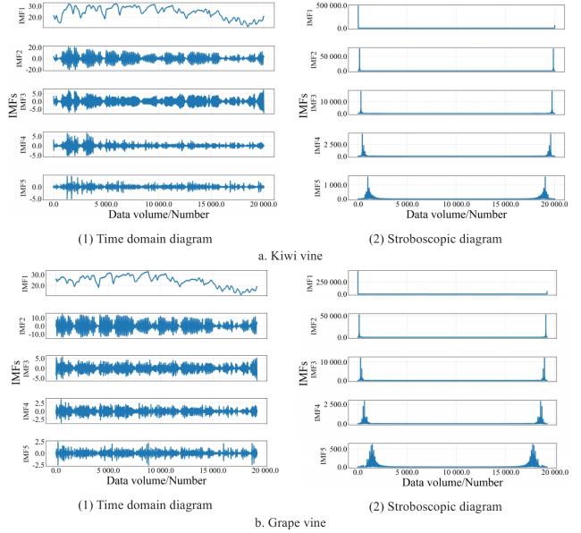
Fig. 11 Time-domain graph and frequency-domain graph of VMD decomposition
The fitness curve keeps converging during the optimization search process using the RIME algorithm, and the result of the converged curve is shown in Fig.12. In Fig.12(a), the minimum fitness value searched after 20 iterations is -1.011 0, at this time, the corresponding parameter combination [K, α] is [14, 2 420], that is, the optimal parameter combination for the decomposition of kiwifruit canopy temperature sequence. Similarly, in Fig. 12(b), the minimum fitness of the grape canopy temperature sequence is -1.342 2, and the optimal parameter combination [K,   α] is [15, 4 000].
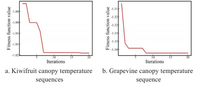
Fig. 12 Convergence curve of fitness values
As shown in Fig. 13, the raw signals of kiwifruit and grape canopy temperatures were processed by the RIME-VMD algorithm to obtain 13 and 15 modal components, respectively. Fig. 13a(1) and Fig. 13b(1) present clearer vibration modes. From the spectra of Fig. 13a(2) and Fig. 13b(2), it can be seen that the signals decomposed by the RIME-VMD method are more independent of each modal center frequency compared with the unoptimized VMD results, which effectively avoids the phenomenon of modal aliasing.
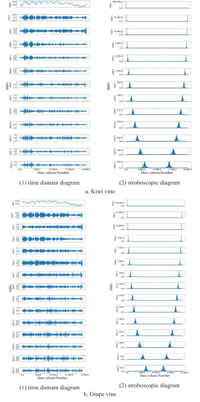
Fig. 13 Time and frequency domain plots of RIME-VMD decomposition

2.4 Ablation experiment

In order to verify the effect of adding VMD decomposition algorithm and RIME optimization algorithm as well as RIME-VMD optimization decomposition method to the LSTM model to improve the prediction accuracy of the model, the ablation test was conducted on RIME2-VMD-LSTM. In the ablation test, the unoptimized LSTM was set to have 100 neurons, 50 rounds, 16 input steps, 64 batch_size, 0.001 learning_rate, 0.1 Dropout, and the prediction test was conducted on the kiwifruit and grape canopy temperature datasets respectively.
The Fig.14 shows the real canopy temperature fitting curve and the prediction curve of each model. The red curve is the real canopy temperature data, the blue is the model prediction curve of this paper, and the rest of the curves represent the baseline models during the experiment, respectively. According to the prediction effect Fig.14, it can be seen that on the 2 sets of data sets, the RIME-LSTM and LSTM models are not effective, and there is an obvious deviation from the true canopy temperature curve. The RIME-VMD-LSTM and VMD-LSTM curves are closer to each other, and the VMD-RIME-LSTM curve is closer to the red curve compared with these 2 curves. The best overall fit to the real canopy temperature curve is the blue curve, i.e. the prediction effect of the optimization model RIME2-VMD-LSTM is the closest to the real data.
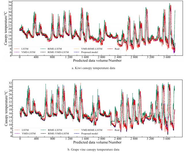
Fig. 14 Prediction performance chart of different models of ablation study
As shown in Table 6, the results of the evaluation indexes of the six models on the kiwifruit and grape canopy temperature datasets, respectively, predicted for the next 1 to 3 hours. It is noted that the RMSE and MAE values all increase with increasing prediction length, while R 2 decreases accordingly. Table 7 shows the results of Table 4 for the mean values of the evaluation metrics on the 2 datasets: For 1-hour predictions, average RMSE = 1.412 6 ℃, MAE = 0.899 0 ℃, and R 2= 0.968 4; for 2-hour predictions, average RMSE= 1.772 4 ℃, MAE = 1.683 2 ℃, and R 2= 0.910 5; for 3-hour predictions, average RMSE = 2.744 9 ℃, MAE = 1.898 8 ℃, and R 2= 0.650 4. Comparatively the proposed model RMSE and MAE have a certain degree of reduction compared to the comparison model, R 2 has a different degree of growth, further calculation of the specific increase or decrease is shown in Table 8 below.
Table 6 Results of ablation experiment of model forecasting study
Temp Comparison models Next 1 hour Next 2 hours Next 3 hours
RMSE/℃ MAE/℃ R 2 RMSE/℃ MAE/℃ R 2 RMSE/℃ MAE/℃ R 2
Kiwi canopy LSTM 1.926 3 1.195 8 0.829 5 2.819 4 1.871 4 0.731 9 4.717 0 2.564 3 0.412 1
VMD-LSTM 1.734 1 1.200 3 0.876 5 2.805 2 1.760 6 0.769 4 4.437 4 2.976 8 0.491 2
RIME-LSTM 1.933 3 1.234 3 0.849 1 2.842 6 1.930 9 0.890 1 4.196 3 2.522 8 0.477 7
RIME-VMD-LSTM 1.708 5 1.174 5 0.879 8 3.205 2 2.125 6 0.756 9 4.548 9 3.005 0 0.347 7
VMD-RIME-LSTM 1.465 8 0.937 9 0.911 7 2.912 4 1.756 9 0.761 6 4.096 6 2.613 6 0.509 6
Proposed model 1.446 6 0.900 7 0.963 9 1.734 1 2.116 0 0.906 3 3.678 9 2.547 1 0.655 9
Grape canopy LSTM 1.860 6 1.259 0 0.841 7 2.997 6 2.099 4 0.648 7 4.038 2 2.926 3 0.425 3
VMD-LSTM 1.610 8 1.194 9 0.923 2 2.734 0 1.936 2 0.663 5 3.753 1 2.611 0 0.465 9
RIME-LSTM 1.810 8 1.250 5 0.884 8 2.772 0 1.837 6 0.653 0 3.937 5 2.666 9 0.299 9
RIME-VMD-LSTM 1.574 5 1.125 0 0.888 1 2.686 4 1.852 2 0.674 1 3.731 2 2.598 4 0.371 4
VMD-RIME-LSTM 1.465 8 0.924 6 0.914 4 2.611 8 1.731 0 0.692 9 4.196 3 2.522 8 0.476 7
Proposed model 1.378 6 0.897 3 0.973 0 1.810 8 1.250 5 0.914 8 1.810 8 1.250 5 0.644 8

Note:Bold values in the table indicate the best performance for each category. Reported RMSE and MAE values represent the mean results across both kiwifruit and grape canopy temperature datasets.

Table 7 Average results of ablation experiments on two kinds of datasets of model forecasting study
Comparison models Next 1 hour Next 2 hours Next 3 hours
RMSE/℃ MAE/℃ R 2 RMSE/℃ MAE/℃ R 2 RMSE/℃ MAE/℃ R 2
LSTM 1.893 5 1.227 4 0.835 6 2.908 5 1.985 4 0.690 3 4.377 6 2.745 3 0.418 7
VMD-LSTM 1.672 4 1.197 6 0.899 8 2.769 6 1.848 4 0.716 5 4.095 2 2.793 9 0.478 6
RIME-LSTM 1.872 1 1.242 4 0.867 0 2.807 3 1.884 2 0.771 6 4.066 9 2.594 8 0.388 8
RIME-VMD-LSTM 1.641 5 1.149 8 0.883 9 2.945 8 1.988 9 0.715 5 4.140 0 2.801 7 0.359 5
VMD-RIME-LSTM 1.465 8 0.931 3 0.913 1 2.762 1 1.744 0 0.727 3 4.146 4 2.568 2 0.493 2
Proposed model 1.412 6 0.899 0 0.968 4 1.772 4 1.683 2 0.910 5 2.744 9 1.898 8 0.650 4

Note:Bold values in the table indicate the best performance for each category. Reported RMSE and MAE values represent the mean results across both kiwifruit and grape canopy temperature datasets.

Table 8 Increase/decrease of indicators between the proposed model and the comparative models of model forecasting study
Comparison models Next 1 hour Next 2 hours Next 3 hours
RMSE/% MAE/% R 2/% RMSE/% MAE/% R 2/% RMSE/% MAE/% R 2/%
LSTM -25.39 -26.75 15.90 -39.06 -15.22 31.91 -37.30 -30.84 55.33
VMD-LSTM -15.53 -24.93 7.62 -36.00 -8.93 27.09 -32.97 -32.04 35.90
RIME-LSTM -24.54 -27.64 11.71 -36.86 -10.67 18.01 -32.51 -26.82 67.28
RIME-VMD-LSTM -13.94 -21.81 9.56 -39.83 -15.37 27.26 -33.70 -32.23 80.89
VMD-RIME-LSTM -3.63 -3.46 6.06 -35.83 -3.48 25.20 -33.80 -26.07 31.87
Negative values in Table 7 indicate decreases in model metrics relative to the comparison model, while positive values indicate increases. Overall, the proposed model delivers more accurate canopy temperature predictions than the others. It significantly reduces RMSE and MAE across both datasets and all three prediction horizons, and it markedly increases R 2 compared to the standard LSTM and the experimental benchmark model. Adding VMD preprocessing to LSTM improves hourly forecasts. For the 1~3 h ahead trials, VMD-LSTM raises R 2 by 7.69%, 3.79%, and 14.30%, respectively, demonstrating the benefit of VMD decomposition. Incorporating RIME optimization into VMD-RIME-LSTM further increases R 2 by 1.47%, 1.51%, and 3.05%, confirming RIME's effectiveness. Compared with VMD-RIME-LSTM, the proposed model achieves lower RMSE and MAE and higher R 2. In the next 2 hours, RMSE drops by 35.83%; in the next 3 hours, MAE falls by 26.07% and R 2 rises by 31.87%, which is the largest improvements of all metrics and horizons. These results validate the efficacy of the RIME-VMD optimization and underscore that each enhancement, including VMD, RIME, and their combination, significantly boosts predictive accuracy.

2.5 Prediction test for different noise environments

In order to assess the robustness of the RIME2-VMD-LSTM canopy temperature prediction model in an unknown time-varying agricultural production environment, as well as to improve the generalization ability of the model. The raw canopy temperature data of kiwifruit and grapes were pre-processed with added noise, including 2 types of noise, uniform, and Gaussian, to simulate the random disturbances generated by the agricultural producers' labor during the data collection process of the real farmland environment and the randomness and uncertainty generated by the weather changes, respectively. RIME2-VMD-LSTM was compared with the classical prediction models Convolutional Neural Network (CNN), Gated Recurrent Unit (GRU), LSTM, and the variant models of LSTM, ConvLSTM, and PC-LSTM, for prediction on 2 datasets of kiwifruit and grape canopy temperatures.
As shown in Table 9, all models performed well on the raw kiwifruit canopy temperature data except ConvLSTM, whose RMSE and MAE were both exceeded 1°C and whose R 2 fell below 0.8. Among the remaining models, the proposed model achieved the lowest values of RMSE and MAE (0.360 1 and 0.254 3°C) and the highest R 2 of 0.994 7, with the CNN model ranking second. After adding uniform noise, all six models saw degraded metrics, but the proposed model suffered the smallest declines and retained an R 2 of 0.929 7. With Gaussian noise, GRU, ConvLSTM, and PC-LSTM produced negative R 2 values, which impaired their fit. This may be introduced by the noise. In contrast, the proposed model's R 2 remained above 0.67, demonstrating the robustness of the proposed model.
Table 9 Comparison of indicators between the proposed model and the comparative models (kiwi)
Models Original data Uniform noise Gaussian noise
RMSE/℃ MAE/℃ R 2 RMSE/℃ MAE/℃ R 2 RMSE/℃ MAE/℃ R 2
CNN 0.497 2 0.316 2 0.990 0 3.347 3 2.794 1 0.657 6 5.548 9 4.416 5 0.372 4
GRU 0.946 0 0.586 6 0.963 7 3.669 9 3.017 0 0.588 4 7.056 5 5.617 2 -0.015 0
LSTM 0.529 8 0.457 0 0.978 5 13.896 2 3.034 6 0.575 3 6.320 2 5.138 7 0.237 4
ConvLSTM 1.150 7 1.521 4 0.798 0 4.003 4 3.246 3 0.510 2 7.170 9 5.696 1 -0.048 1
PC-LSTM 0.779 1 0.601 0 0.975 4 4.050 9 3.271 2 0.498 5 7.592 3 6.008 1 -0.174 9
Proposed model 0.360 1 0.254 3 0.994 7 1.501 0 1.214 2 0.929 7 3.885 5 3.080 7 0.678 9

Note:Bold values in the table indicate the best performance for each category. Reported RMSE and MAE values represent the mean results across both kiwifruit and grape canopy temperature datasets.

As can be seen from Table 9 and Table 10, when testing with uniform and Gaussian noise added to the canopy temperature data for single-step predictions, the model achieved average RMSE values of 1.265 2 ℃ and 2.975 3 ℃, MAE values of 1.016 1 ℃ and 2.368 8 ℃, and R 2 values of 0.945 5 and 0.791 2, respectively (all values derived from raw data in Table 9 and Table 10). Although the model's performance metrics show decreases when applied to noise-added data compared to original data, it still maintains the lowest RMSE, MAE, and highest R 2 among all comparison models. Notably, the R 2 remains above 0.90 for the uniform noise condition.
Table 10 Comparison of indicators between the proposed model and the comparative models (grape)
Models Original data Uniform noise Gaussian noise
RMSE/℃ MAE/℃ R 2 RMSE/℃ MAE/℃ R 2 RMSE/℃ MAE/℃ R 2
CNN 0.525 4 0.344 4 0.987 8 3.999 9 3.230 0 0.486 5 5.860 3 4.663 9 0.297 0
GRU 1.092 1 0.730 6 0.947 2 4.221 0 3.409 7 0.428 2 7.484 9 6.001 6 -0.146 8
LSTM 3.321 1 1.029 0 0.853 1 18.878 4 3.516 5 0.394 1 54.543 2 5.919 4 -0.116 5
ConvLSTM 1.646 0 1.145 8 0.880 2 6.559 2 5.034 7 -0.380 9 7.622 9 6.137 6 -0.189 5
PC-LSTM 0.889 3 0.669 8 0.965 0 4.778 1 3.864 1 0.267 3 8.596 2 6.878 1 -0.512 7
Proposed model 0.287 0 0.185 7 0.996 3 1.029 4 0.817 9 0.961 3 2.065 0 1.656 8 0.903 4

Note:Bold values in the table indicate the best performance for each category. Reported RMSE and MAE values represent the mean results across both kiwifruit and grape canopy temperature datasets.

The experimental results show that the proposed model has a good prediction effect on the original data of kiwifruit and grape canopy temperature, the data with added noise to simulate the environmental disturbances, and the proposed model has low sensitivity to the disturbing noise, which verifies the robustness of the proposed model, and further verifies the validity of the canopy temperature prediction model of RIME2-VMD-LSTM.

3 Conclusions

This paper proposed a canopy temperature prediction model named RIME2-LSTM-VMD, which integrates the LSTM neural network, VMD, and the RIME optimization algorithm. The model is designed to address the challenge of predicting canopy temperature in kiwifruit and grape production within agricultural demonstration orchards. Firstly, a combined model for canopy temperature prediction was constructed based on the LSTM neural network and five temporal data decomposition methods (EMD, CEEMDAN, VMD, SGMD, and TVF-EMD). The optimal base model, VMD-LSTM, was selected. Secondly, five optimization algorithms (PSO, SSA, GWO, SAO, and RIME) were employed on the base model to optimize the LSTM main parameters, construct the optimization model, and add the RIME-VMD optimization decomposition algorithm. The final result of this study is the RIME2-VMD-LSTM canopy temperature prediction model. Experimental results demonstrate that: For the next 1~3 hour canopy temperature predictions of kiwifruit and grape, the proposed model demonstrates statistically significant reductions in RMSE and MAE, coupled with notable improvements in R 2 against baseline models. Under simulated noisy conditions, the model exhibits superior robustness with RMSE (0.360 1 ℃), MAE (0.254 3 ℃), and R 2 (0.994 7) outperforming all comparison methods. These results validate both the effectiveness and robustness of this model. For future work, further optimization of the model is planned to enhance its robustness.

All authors declare no competing interests.

[1]
ZHANG Q Y, YANG X Z, LIU C, et al. Monitoring soil moisture in winter wheat with crop water stress index based on canopy-air temperature time lag effect[J]. International journal of biometeorology, 2024, 68(4): 647-659.

[2]
WANG X L, LUO N, ZHU Y P, et al. Water replenishment to maize under heat stress improves canopy temperature and grain filling traits during the reproductive stage[J]. Agricultural and forest meteorology, 2023, 340: ID 109627.

[3]
JEON Y, CHO L, PARK S, et al. Canopy temperature and heat flux prediction by leaf area index of bell pepper in a greenhouse environment: Experimental verification and application[J]. Agronomy, 2022, 12(8): ID 1807.

[4]
SHAO Q X, BANGE M, MAHAN J, et al. A new probabilistic forecasting model for canopy temperature with consideration of periodicity and parameter variation[J]. Agricultural and forest meteorology, 2019, 265: 88-98.

[5]
YANG M X, GAO P, ZHOU P, et al. Simulating canopy temperature using a random forest model to calculate the crop water stress index of Chinese Brassica [J]. Agronomy, 2021, 11(11): ID 2244.

[6]
ANDRADE M A, O'SHAUGHNESSY S A, EVETT S R. Forecasting of canopy temperatures using machine learning algorithms[J]. Journal of the asabe, 2023, 66(2): 297-305.

[7]
KONDO R, TANAKA Y, SHIRAIWA T. Predicting rice (Oryza sativa L.) canopy temperature difference and estimating its environmental response in two rice cultivars, 'Koshihikari' and 'Takanari', based on a neural network[J]. Plant production science, 2022, 25(3): 394-406.

[8]
YOSHIMOTO M, FUKUOKA M, TSUJIMOTO Y, et al. Monitoring canopy micrometeorology in diverse climates to improve the prediction of heat-induced spikelet sterility in rice under climate change[J]. Agricultural and forest meteorology, 2022, 316: ID 108860.

[9]
BANERJEE S, SINGAL G, SAHA S, et al. Machine Learning approach to Predict net radiation over crop surfaces from global solar radiation and canopy temperature data[J]. International journal of biometeorology, 2022, 66(12): 2405-2415.

[10]
HAIDER SALI, NAQVI S R, AKRAM T, et al. LSTM neural network based forecasting model for wheat production in Pakistan[J]. Agronomy, 2019, 9(2): ID 72.

[11]
TIAN H R, WANG P X, TANSEY K, et al. An LSTM neural network for improving wheat yield estimates by integrating remote sensing data and meteorological data in the Guanzhong Plain, PR China[J]. Agricultural and forest meteorology, 2021, 310: ID 108629.

[12]
KIRAN KUMAR V, RAMESH K V, RAKESH V. Optimizing LSTM and Bi-LSTM models for crop yield prediction and comparison of their performance with traditional machine learning techniques[J]. Applied intelligence, 2023, 53(23): 28291-28309.

[13]
ZHANG J, WU P L, XU X, et al. PCS-LSTM: A hybrid deep learning model for multi-stations joint temperature prediction based on periodicity and closeness[J]. Neurocomputing, 2022, 501: 151-161.

[14]
PANG C, CHENG C, LIU Z J, et al. Prediction of world temperature based on PSO optimized LSTM neural network[C]// 2023 IEEE 3rd International Conference on Information Technology, Big Data and Artificial Intelligence (ICIBA). Piscataway, New Jersey, USA: IEEE, 2023: 125-130.

[15]
PIERRE A A, AKIM S A, SEMENYO A K, et al. Peak electrical energy consumption prediction by ARIMA, LSTM, GRU, ARIMA-LSTM and ARIMA-GRU approaches[J]. Energies, 2023, 16(12): ID 4739.

[16]
WANG A N, QIN P, SUN X M, et al. An automatic parameter setting variational mode decomposition method for vibration signals[J]. IEEE transactions on industrial informatics, 2024, 20(2): 2053-2062.

[17]
WU J H, HU Y, WU D Q, et al. An aquatic product price forecast model using VMD-IBES-LSTM hybrid approach[J]. Agriculture, 2022, 12(8): ID 1185.

[18]
NIU H L, XU K L, WANG W Q. A hybrid stock price index forecasting model based on variational mode decomposition and LSTM network[J]. Applied intelligence, 2020, 50(12): 4296-4309.

[19]
HOU S, GENG Q K, HUANG Y R, et al. Rainfall prediction model based on CEEMDAN-VMD-BiLSTM network[J]. Water, air, & soil pollution, 2024, 235(8): ID 482.

[20]
ZHU Y J, DU W S, WANG C Y, et al. Rapid recognition and picking points automatic positioning method for table grape in natural environment[J]. Smart agriculture, 2023, 5(2): 23-34.

[21]
SU H, ZHAO D, HEIDARI A A, et al. RIME: A physics-based optimization[J]. Neurocomputing, 2023, 532: 183-214.

[22]
NINANYA J, RAMÍREZ D A, RINZA J, et al. Canopy temperature as a key physiological trait to improve yield prediction under water restrictions in potato[J]. Agronomy, 2021, 11(7): ID 1436.

[23]
CHEN P, WANG R, YAO Y B, et al. A short-term prediction model of global ionospheric VTEC based on the combination of long short-term memory and convolutional long short-term memory[J]. Journal of geodesy, 2023, 97(5): ID 51.

[24]
YANG H, YANG X D, LI G H. Forecasting carbon price in China using a novel hybrid model based on secondary decomposition, multi-complexity and error correction[J]. Journal of cleaner production, 2023, 401: ID 136701.

[25]
JAMEI M, ALI M, MALIK A, et al. Development of a TVF-EMD-based multi-decomposition technique integrated with Encoder-Decoder-Bidirectional-LSTM for monthly rainfall forecasting[J]. Journal of hydrology, 2023, 617: ID 129105.

文章导航

/