


0 Introduction
1 Materials and methods
1.1 Data preparation
1.1.1 Safflower picking robot and working principle
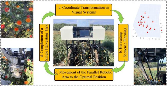
Fig. 1 Flowchart of safflower picking by parallel robot |
1.1.2 Safflower data
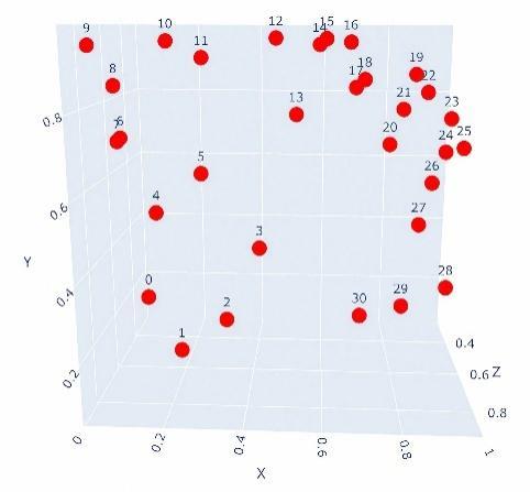
Table 1 Spatial distribution and 3D coordinates of 25 safflower targets |
| Spatial distribution | Lable | Coordinate points | Lable | Coordinate points |
|---|---|---|---|---|
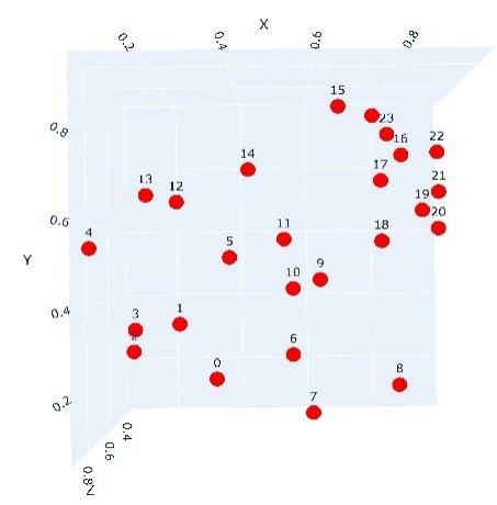 | 1 | (0.370 85, 0.225 16, 0.845 60) | 14 | (0.107 30, 0.718 10, 0.351 90) |
| 2 | (0.2607 1, 0.3415 2, 0.684 10) | 15 | (0.444 20, 0.735 80, 0.791 80) | |
| 3 | (0.150 57, 0.274 46, 0.719 60) | 16 | (0.668 30, 0.909 50, 0.713 80) | |
| 4 | (0.083 69, 0.296 23, 0.402 10) | 17 | (0.829 70, 0.785 10, 0.691 60) | |
| 5 | (0.091 51, 0.540 71, 0.899 40) | 18 | (0.773 30, 0.714 30, 0.719 50) | |
| 6 | (0.407 40, 0.517 10, 0.910 40) | 19 | (0.794 20, 0.560 00, 0.591 80) | |
| 7 | (0.549 00, 0.278 40, 0.820 40) | 20 | (0.896 50, 0.643 30, 0.628 80) | |
| 8 | (0.608 00, 0.065 50, 0.524 90) | 21 | (0.942 30, 0.594 00, 0.613 50) | |
| 9 | (0.820 50, 0.177 80, 0.694 80) | 22 | (0.938 50, 0.692 60, 0.634 90) | |
| 10 | (0.619 90, 0.457 80, 0.710 90) | 23 | (0.968 60, 0.824 70, 0.490 60) | |
| 11 | (0.551 69, 0.434 36, 0.694 90) | 24 | (0.841 50, 0.897 50, 0.391 80) | |
| 12 | (0.529 40, 0.564 48, 0.701 90) | 25 | (0.801 60, 0.962 40, 0.361 80) | |
| 13 | (0.284 33, 0.649 31, 0.872 60) |
Table 3 Spatial distribution and 3D coordinates of 43 safflower targets |
| Spatial distribution | Lable | Coordinate points | Lable | Coordinate points |
|---|---|---|---|---|
| | 1 | (0.066 90, 0.944 80, 0.220 69) | 23 | (0.958 28, 0.501 20, 0.077 57) |
| 2 | (0.272 09, 0.007 86, 0.789 90) | 24 | (0.978 76, 0.869 70, 0.144 32) | |
| 3 | (0.291 00, 0.675 90, 0.498 20) | 25 | (0.413 78, 0.755 43, 0.050 40) | |
| 4 | (0.274 50, 0.580 01, 0.828 09) | 26 | (0.280 54, 0.011 32, 0.336 20) | |
| 5 | (0.387 98, 0.546 18, 0.486 30) | 27 | (0.236 89, 0.745 04, 0.409 20) | |
| 6 | (0.026 03, 0.840 90, 0.239 20) | 28 | (0.970 50, 0.141 88, 0.509 40) | |
| 7 | (0.017 18, 0.414 45, 0.101 10) | 29 | (0.881 24, 0.569 85, 0.649 90) | |
| 8 | (0.927 67, 0.631 05, 0.318 80) | 30 | (0.582 91, 0.902 41, 0.734 50) | |
| 9 | (0.371 76, 0.72219, 0.901 90) | 31 | (0.662 84, 0.021 60, 0.092 40) | |
| 10 | (0.269 97, 0.768 43, 0.741 02) | 32 | (0.204 40, 0.369 01, 0.800 06) | |
| 11 | (0.725 02, 0.085 77, 0.862 82) | 33 | (0.169 60, 0.898 20, 0.854 90) | |
| 12 | (0.559 95, 0.614 29, 0.183 17) | 34 | (0.839 21, 0.173 10, 0.265 33) | |
| 13 | (0.884 94, 0.752 67, 0.490 53) | 35 | (0.513 48, 0.998 80, 0.585 30) | |
| 14 | (0.783 94, 0.016 53, 0.096 84) | 36 | (0.033 25, 0.672 79, 0.615 30) | |
| 15 | (0.787 99, 0.435 66, 0.371 51) | 37 | (0.549 80, 0.890 58, 0.660 40) | |
| 16 | (0.122 35, 0.477 45, 0.504 56) | 38 | (0.298 60, 0.111 27, 0.308 30) | |
| 17 | (0.297 22, 0.291 65, 0.551 51) | 39 | (0.636 40, 0.499 50, 0.296 30) | |
| 18 | (0.321 45, 0.471 07, 0.879 74) | 40 | (0.824 54, 0.998 80, 0.981 20) | |
| 19 | (0.831 73, 0.542 33, 0.048 44) | 41 | (0.971 44, 0.608 50, 0.847 90) | |
| 20 | (0.105 04, 0.866 72, 0.470 37) | 42 | (0.372 60, 0.688 90, 0.952 72) | |
| 21 | (0.048 52, 0.678 90, 0.475 20) | 43 | (0.611 60, 0.412 78, 0.091 30) | |
| 22 | (0.344 70, 0.201 90, 0.167 13) |
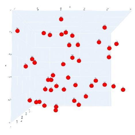
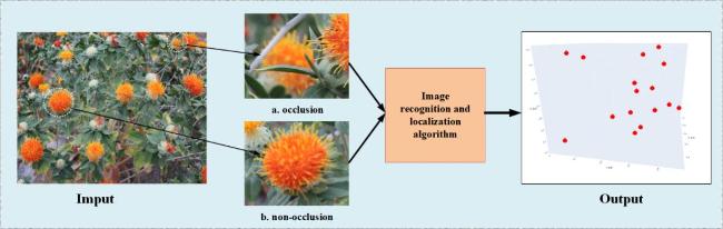
Fig. 2 Workflow of vision-based safflower recognition and localization system |
Table 2 Spatial distribution and 3D coordinates of 31 safflower targets |
| Spatial distribution | Lable | Coordinate points | Lable | Coordinate points |
|---|---|---|---|---|
| | 1 | (0.031 29, 0.153 36, 0.352 20) | 17 | (0.670 69, 0.953 60, 0.498 40) |
| 2 | (0.195 88, 0.113 25, 0.634 10) | 18 | (0.676 65, 0.848 85, 0.684 30) | |
| 3 | (0.345 74, 0.266 43, 0.769 10) | 19 | (0.701 89, 0.865 28, 0.642 40) | |
| 4 | (0.417 69, 0.398 49, 0.586 40) | 20 | (0.797 98, 0.896 00, 0.891 50) | |
| 5 | (0.170 80, 0.548 25, 0.781 10) | 21 | (0.766 78, 0.708 47, 0.688 10) | |
| 6 | (0.273 79, 0.629 54, 0.697 40) | 22 | (0.812 71, 0.784 00, 0.581 70) | |
| 7 | (0.100 57, 0.739 19, 0.826 40) | 23 | (0.853 47, 0.841 81, 0.724 50) | |
| 8 | (0.024 39, 0.693 11, 0.597 60) | 24 | (0.944 39, 0.759 25, 0.573 90) | |
| 9 | (0.092 73, 0.861 65, 0.837 10) | 25 | (0.919 31, 0.683 73, 0.649 20) | |
| 10 | (0.051 98, 0.953 60, 0.887 40) | 26 | (0.968 68, 0.692 05, 0.637 40) | |
| 11 | (0.187 26, 0.958 50, 0.682 74) | 27 | (0.878 55, 0.613 11, 0.695 20) | |
| 12 | (0.264 38, 0.914 77, 0.599 40) | 28 | (0.852 53, 0.497 48, 0.673 30) | |
| 13 | (0.473 02, 0.967 90, 0.726 40) | 29 | (0.971 19, 0.255 98, 0.488 40) | |
| 14 | (0.527 73, 0.798 08, 0.822 40) | 30 | (0.812 71, 0.277 10, 0.683 30) | |
| 15 | (0.582 28, 0.953 60, 0.742 70) | 31 | (0.730 42, 0.069 73, 0.268 40) | |
| 16 | (0.599 52, 0.966 62, 0.705 60) |
1.2 Combinatorial optimization problem formulation
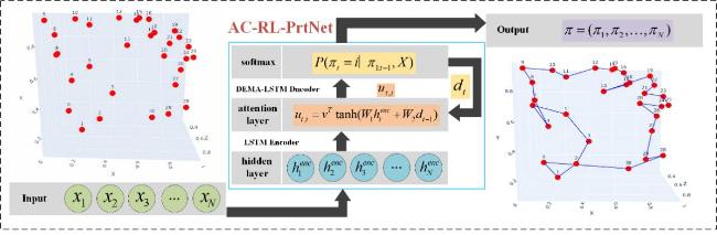
Fig. 3 The process of modelling input to output of AC-RL-PrtNet |
1.3 Overview of the RL pointer network based on the Actor-Critic architecture
1.3.1 Encoder-decoder architecture
Table 4 Ablation results for hidden state dimension |
| Hidden dim | Training time/s | Best path | Model size/MB |
|---|---|---|---|
| 64 | 1 672 | 11.856 | 4.251 |
| 128 | 1 998 | 11.414 | 4.462 |
| 256 | 2 920 | 11.186 | 5.282 |
1.3.2 MDPmodeling
1.3.3 Policy gradient method
1.3.4 Actor-Critic architecture and policy
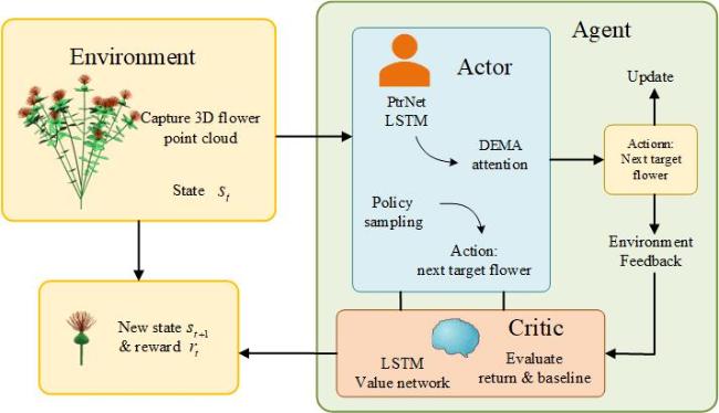
Fig. 4 An interactive Actor-Critic decision framework for 3D safflower picking tasks |
2 Algorithm improvement
2.1 Dynamic exponential moving average attention mechanism
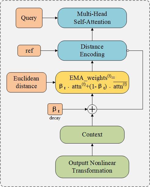
Fig. 5 Computational flow of the DEMA attention mechanism |
2.1.1 Redefinition of multi head self attention
2.1.2 Incorporation of distance encoding
2.1.3 Adaptive EMA weight adjustment
2.1.4 Nonlinear transformation of output
2.2 Network pruning
2.2.1 LSTM gate importance based pruning strategy
2.2.2 Structured pruning implementation for gate structures
2.3 Structural enhancements of the critic network
2.3.1 Enhanced input embedding with normalization mechanisms
2.3.2 Contextual aggregation from LSTM encoder
2.3.3 Lightweight attention-based context fusion
2.4 Algorithm learning method
| Training Algorithm |
|---|
| Input: Number of training iterations S, batch size B |
| Output: Optimal path Initialize: (with internal dynamic EMA attention module), , Optimizer and learning rate |
| for t= 1 to S do: |
| The Actor network generates B trajectories via a DEMA-based attention mechanism:
|
| Compute reward R(π) and log-probability:
|
| Value estimation using the Critic network:
|
| Compute advantage:
|
| Update Actor: Backpropagate the error through the LSTM-based DEMA module in the Actor network:
|
| Update Critic using mean-squared error loss:
|
| end for: Return to the shortest path |
3 Experiments and results
3.1 Impact of DEMA on the model
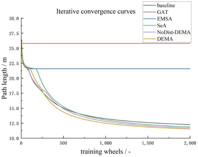
Fig. 6 Iterative convergence comparison of various attention mechanisms against the baseline |
Table 5 Comparison of results of different architectures under various numbers of safflower points |
| Method | n=20 | n=28 | n=37 | n=46 | ||||
|---|---|---|---|---|---|---|---|---|
| Length /cm | Time/s | Length/cm | Time /s | Length/cm | Time/s | Length /cm | Time/s | |
| baseline | 6.769 | 90.83 | 8.524 | 183.26 | 10.299 | 368.36 | 11.806 | 511.05 |
| GAT | 7.399 | 98.46 | 12.064 | 197.85 | 16.638 | 414.79 | 23.665 | 602.34 |
| EMSA | 8.321 | 126.12 | 11.992 | 254.96 | 15.251 | 496.07 | 19.019 | 582.41 |
| SeA | 6.675 | 63.07 | 8.404 | 185.84 | 9.940 | 327.68 | 11.433 | 510.73 |
| NoDist-DEMA | 6.719 | 59.32 | 8.346 | 123.94 | 10.145 | 231.76 | 11.402 | 304.78 |
| DEMA | 6.674 | 51.01 | 8.302 | 113.74 | 10.058 | 224.29 | 11.398 | 334.62 |
|
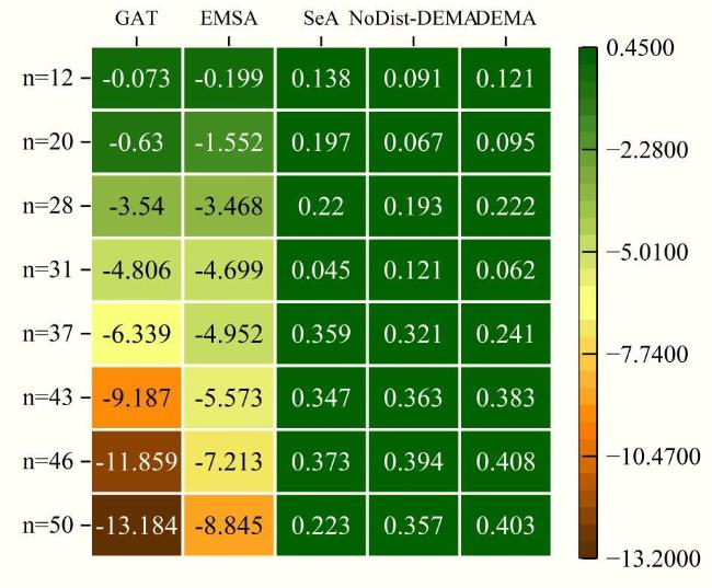
Fig. 7 Path length gap of different models at different test points |
3.2 Impact of pruning on the model
Table 6 Comparison of results for different pruning strategies of the proposed model |
| Strategy | Encoder pruning | Decoder pruning | Params | Sparsity/% | Training Time/s | Speedup/% | |||
|---|---|---|---|---|---|---|---|---|---|
| Input gate | Output gate | Input gate | Output gate | Initial (×105) | Modified (×105) | ||||
| Group A | 0.35 | 0.35 | 0.35 | 0.35 | 4.462 | 4.106 | 8 | 161 | —— |
| Group B | 0.25 | 0.25 | 0.25 | 0.25 | 4.265 | 4.44 | 1 747 | 12 | |
| Group C | 0.35 | 0.35 | 0.25 | 0.25 | 4.201 | 5.88 | 1 698 | 15 | |
|
3.3 Ablation study on model enhancements
Table 7 Ablation study on model enhancements |
| baseline | DEMA | Pruning | The enhanced Critic | n=25 | n=31 | n=43 | |||
|---|---|---|---|---|---|---|---|---|---|
| Length/cm | Time/s | Length/cm | Time/s | Length/cm | Time/s | ||||
| √ | 6.674 | 88.08 | 6.749 | 167.35 | 11.426 | 497.50 | |||
| √ | 5.930 | 80.86 | 6.647 | 127.00 | 11.049 | 262.47 | |||
| √ | √ | 5.907 | 63.00 | 6.441 | 125.00 | 11.043 | 244.27 | ||
| √ | √ | √ | 5.826 | 69.79 | 6.356 | 94.90 | 10.784 | 244.50 | |
3.4 Comparison with swarm intelligence algorithms
Table 8 Comparison of the proposed AC-RL-PtrNet model with traditional algorithms |
| Method | n=25 | n=31 | ||||||
|---|---|---|---|---|---|---|---|---|
| Length/cm (p-value) | Improvement rate/% | Time/s | Improvement Rate/% | Length /cm (p-value) | Improvement rate/% | Time/s | Improvement Rate/% | |
| Baseline | 6.084(p<0.008 0) | 4.24 | 82.00 | 14.85 | 6.913 0(p<0.005) | 8.07 | 215.0 | 55.86 |
| PSO | 15.123 (p<0.001 0) | 61.47 | 183.00 | 61.87 | 15.437 5 (p<0.001) | 58.82 | 232.0 | 59.10 |
| ACO | 7.09(p<0.001 0) | 17.84 | 104.00 | 32.91 | 6.966 2(p<0.001) | 8.75 | 123.0 | 22.93 |
| NSGA | 6.44(p<0.003 6) | 9.56 | 68.00 | -2.63 | 7.960 0(p<0.001) | 20.17 | 135.0 | 29.70 |
| AC-RL-PtrNet | 5.826 | — | 69.79 | — | 6.356 0 | — | 94.9 | — |
|
3.5 Field experiment
3.5.1 Field setup and real-world planning examples
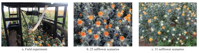
Fig. 8 Field experiment setup and example planning results for 25 and 31 safflower blossoms |
3.5.2 Analysis of sequence planning results
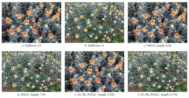
Fig. 9 Comparison of safflower picking sequence planning on 25 and 31 flowers |


