


0 Introduction
Soybean yield prediction using remote sensing relies on the spectral response of crops at canopy level[1], so model quality directly determines how reliable the final numbers are[2]. Yet high accuracy and broad coverage are hard to get from a single platform. Unmanned aerial vehicles (UAV) fly low, capture fine spatial detail, but can only cover a few plots at a time; scaling them up to a whole farm or county is practically impossible. Satellites, on the other hand, do cover large areas in one pass, yet cloud, haze and fog routinely spoil the images, and fixed revisit cycles mean a clear shot may not be obtained exactly when needed [3].
With the push of remote sensing technology, researchers now have access to images of many spatial, spectral and temporal flavors for the same area—which called multi-source remote sensing datasets[4]. LIAO et al.[5] fused Landsat-8 and MODIS data in eastern Ontario for soybean yield estimation, but their work stayed at field scale. WANG et al.[6] used the Spatial and Temporal Non-Local Filter-based Fusion Model to blend Sentinel-2A and MODIS observations for summer maize simulation, achieving an R 2 of 0.84. YANG et al.[7] fused RGB, multispectral and thermal UAV imagery for wheat yield prediction; their best combination (RGB-MS-Texture-TIR) reached R 2=0.660, RMSE (Root Mean Square Error)=0.754. These results showed promise, yet each had its blind spot: satellite-only fusion still carried geometric, spectral and spatial mismatches that blunt prediction accuracy; UAV-only setups delivered detail but cannot step up to regional monitoring. YANG[8] built a UAV-satellite cross-scale system for potato growth parameter retrieval, using UAV-derived pixel-level data to calibrate satellite models. That idea is clever, yet it was tailored to potatoes, and crop-specific phenology and spectral traits make it hard to port straight to soybean. Overall, UAV-satellite fusion work is still sparse, and resolution gaps have largely blocked effective integration.
VAN HOUT [9] showed that crops change continuously through the season, so a single snapshot misses the dynamics. ZHOU et al.[10] and HAN et al.[11] used trapezoidal integration of multi-temporal vegetation indices to show that UAV-based multi-date indices boost rice and summer maize yield estimates well beyond single-stage data LU et al.[12] conducted correlation analyses between diverse vegetation indices across multiple temporal acquisitions and winter wheat yield, revealing that correlation magnitude progressively strengthened concomitant with phenological advancement, attaining a zenith of 0.7 during the booting stage (March 26). ZHAO et al.[13] leveraged multi-temporal canopy multispectral UAV imagery from 266 wheat cultivars to construct yield prediction models incorporating both single- and multi-stage phenological information, with optimal performance achieved by a Random Forest model based on five growth stages, yielding a predictive R 2 of 0.834. Accordingly, utilization of multi-temporal remote sensing data constitutes a prerequisite for improving crop yield estimation precision. Nonetheless, systematic and in-depth investigation into the optimal selection of temporal granularity and configuration of temporal combination strategies remains scarce[14].
However, despite the above achievements, several critical issues still restrict the accuracy and applicability of soybean yield estimation. First, the contradiction between high precision and large-scale monitoring remains unsolved: UAV data provides fine details but lacks regional coverage, while satellite data achieves wide coverage but suffers from cloud contamination and coarse resolution. Second, most existing studies ignore the optimal selection of temporal granularity and lack quantitative comparisons between different time windows, leading to incomplete capture of crop growth dynamics. Third, current multi-source fusion methods mostly stay at the level of data splicing, failing to realize deep feature fusion and temporal dependency modeling, resulting in limited model performance. To address these gaps, a high-precision soybean yield estimation framework is constructed in this study based on UAV-Sentinel-2 multi-source data fusion, with the aim of achieving effective spatiotemporal matching, deep feature integration and accurate large-scale yield prediction.
A multi-source data fusion algorithm was adopted to integrate UAV and satellite multi-temporal remote sensing observations in this study, on the basis of which an enhanced convolutional neural network (CNN) framework for soybean yield estimation was developed. By systematically evaluating the effects of diverse fusion methodologies and critical temporal phases on model performance, the optimal fusion strategy and most informative phenological windows were identified, thereby facilitating accurate soybean yield forecasting for Jianshan Farm.
1 Materials and methods
1.1 Study area
Field experiments were carried out at Jianshan Farm, Heihe, Heilongjiang-a core soybean-producing zone referred to as China's "Soybean Capital". The farm spans 125°19′53″E-125°47′15″E and 48°46′55″N-49°1′18″N, with annual precipitation of roughly 500-600 mm falling mostly in July and August. Its cold-temperate continental monsoon climate and contiguous, ridge-based cultivation pattern make it representative of large-scale mechanised soybean production in Northeast China.
1.2 Data
1.2.1 Field data acquisition
Field data surveys were conducted in the experimental area of Jianshan Farm to ensure the accuracy of data annotation during remote sensing image processing. The sample was conducted from September 15th to September 30th, 2022, and from September 5th to September 13th, 2023. The main focus was on collecting yield information from four plots: North 13 Plot,North 14 Plot,North 15 Plot,and North 9 Plot (North 13 Plot,North 14 Plot,North 15 Plot,andNorth 9 Plot), with corresponding areas of 50.4, 55.4, 53.4, and 51.2 hm2, respectively, totaling 210.4 hm2. Manual sampling was conducted using a grid method, with five sampling points per grid (Fig. 1), and the latitude and longitude information along with the yield of each point were recorded. Specifically, 194 sampling points were collected in North 13 Plot, 195 in North 14 Plot, 180 in North 15 Plot, and 201 in North 9 Plot, totaling 770 sampling points. For each sampling point, an area of 1 m2 was selected to count the total number of soybean plants and the number of pods on each plant. The total number of soybeans within the area was calculated, and the hundred-grain weight of soybeans was obtained using a balance. Finally, soybean yield was calculated using the Equation(1) .
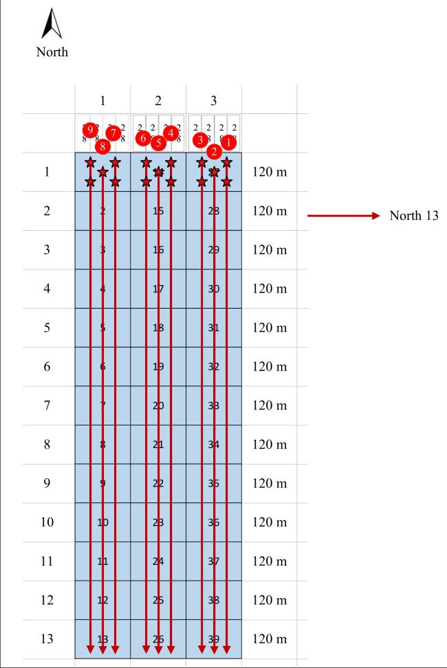
Fig. 1 Five-point sampling combined with grid method for soybean field survey at Jianshan Farm |
Where, T represents yield, kg/hm2; S represents the number of grains per plant, grains; B represents the total number of plants, individuals; and Q represents the hundred-grain weight, kg.
1.2.2 Sentinel-2 imagery acquisition and preprocessing
A total of 124 Sentinel-2 imagery data from the years 2022 to 2023 (Table 1) was selected, excluding three bands (1, 9, and 10) with a resolution of 60 m. Only the remaining nine bands of the Sentinel-2 were studied. It can be observed from Table 1 that during the entire growth period of soybeans at Jianshan Farm, the Sentinel-2 passed over the area every 2 to 3 days.
Table 1 Band information of acquired Sentinel-2 imagery |
| Band number | Band | Central wavelength/μm | Bandwidth/nm | Spatial resolution/m |
|---|---|---|---|---|
| 1 | Coastal aerosol | 0.443 | 20 | 60 |
| 2 | Blue | 0.490 | 65 | 10 |
| 3 | Green | 0.560 | 35 | 10 |
| 4 | Red | 0.665 | 30 | 10 |
| 5 | Vegetation red edge | 0.705 | 15 | 20 |
| 6 | Vegetation red edge | 0.740 | 15 | 20 |
| 7 | Vegetation red edge | 0.783 | 20 | 20 |
| 8 | Near Infrared | 0.842 | 115 | 10 |
| 8A | Vegetation red edge | 0.865 | 20 | 20 |
| 9 | Water vapour | 0.945 | 20 | 60 |
| 10 | Short-Wave Infrared -Cirrus | 1.375 | 20 | 60 |
| 11 | SWIR | 1.610 | 90 | 20 |
The preprocessing of Sentinel-2 remote sensing imagery included radiometric calibration, atmospheric correction, and image cropping. Radiometric calibration was performed using the Sen2Cor processor, while atmospheric correction and resolution unification were carried out using SNAP software. Coordinate system settings and image cropping were done in ArcGIS, resulting in the preprocessed Sentinel-2 imagery of the experimental area.
1.2.3 UAV imagery acquisition and preprocessing
The UAV selected was the Da-Jiang Innovations(DJI) Phantom 4 Multispectral (P4M), manufactured by China's DJI company. The data acquisition period covered the entire growth stage of soybeans. Flights were conducted only under clear-sky conditions with wind speeds≤3 m/s to meet solar-elevation requirements and ensure sufficient radiance; image acquisition was scheduled between 10:00-11:30 a.m. or 1:30-2:30 p.m. each day. A total of 47 images were acquired.
When collecting multispectral UAV imagery of soybeans, various factors may interfere, necessitating preprocessing[15]. Pix4D mapper was used for image stitching, which included completeness verification, high-precision alignment, and parameter configuration, enabling automated processing. Subsequently, radiometric correction was performed to convert digital counts into surface radiance or reflectance[16]. The results of radiometric correction using ENVI 5.3 (64-bit) software are shown in Fig. 2, enhancing image quality. Finally, the images were cropped to remove non-study areas and ensure data integrity.
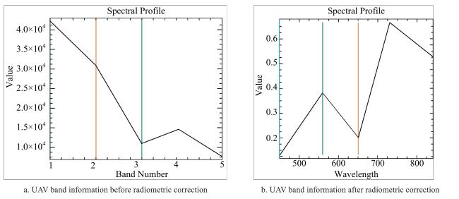
Fig. 2 Comparison of UAV multispectral band information before and after radiometric correction |
Fig. 2a presents the multispectral band information before radiometric correction. Despite the horizontal axis ranging from 1 to 5, there were noticeable deviations in the reflectance values on the vertical axis. Additionally, the bands were arranged in a disordered manner, not in ascending order of wavelength. The horizontal axis in the figure represents the band number, not the specific wavelength. Fig. 2b displays the spectral data after radiometric correction. The corrected data more accurately reflected the reflectance of ground objects, and the band order has been appropriately adjusted to align closely with the spectral curve of the soybean canopy, demonstrating the remarkable effectiveness of the radiometric correction.
1.3 Feature extraction from remote sensing imagery
UAV and Sentinel-2 acquisitions rarely coincided exactly[17], and Sentinel-2 scenes were frequently degraded by cloud cover[18]. Therefore, the multi-temporal was composited to narrow the temporal gap between the two sensors while retaining only clear Sentinel-2 observations[19]. The Savitzky-Golay filter (SGFA) was applied to both datasets to generate half-monthly and monthly synthetic images. A half-monthly window tracked rapid canopy changes-particularly during vegetative growth and pod filling, when spectral signals shifted abruptly-whereas a monthly window smoothed out ephemeral weather noise and captured the broader growth trajectory. Used jointly, they preserved phenological detail without sacrificing long-term stability. SGFA fitted a local polynomial inside a sliding window (third order, nearest-boundary mode, three time steps), which ironed out residual registration errors and suppressed cloud-induced outliers. The output was a pair of temporally consistent image stacks ready for feature extraction.
SGFA smoothing was performed on seven vegetation-index time series-Normalized Difference Vegetation Index (NDVI), Enhanced Vegetation Index (EVI) and Green Normalized Difference Vegetation Index (GNDVI) among them-using the settings above. High-frequency noise was dampened, yet the inflection points of the growth curve remained intact. Cloud screening relied on the Sentinel-2 QA60 band: any scene with >30 % cloud cover was dropped entirely; for scenes at ≤30 %, only cloud-free pixels were averaged. UAV shadows were masked manually. Missing half-monthly slots were filled by linear interpolation provided at least one adjacent phase remained; pixels lacking two or more consecutive values were removed. These rules kept the time series both complete and trustworthy.
Table 2 GLCM texture parameters and their physical significance for soybean canopy characterization |
| Texture feature parameters | Abbreviation | Central band/μm |
|---|---|---|
| Mean texture | Mean | Describe the brightness and darkness of an image |
| Homogeneity texture | Hom | Evaluate the local grayscale uniformity of the image |
| Dissimilarity texture | Dis | Characterize the differences in texture features between pixels |
| Entropy texture | Ent | Indicate the size of the amount of information |
| Second Moment texture | Sm | Describe the uniformity and thickness of texture features |
| Correlation texture | Corr | Predict the main trend of texture |
In Python 3.8 environment, texture feature extraction was conducted on remote sensing images. Firstly, the original remote sensing images were converted to grayscale, from which five key dimensions were separately extracted. To simplify the complexity of subsequent processing, the grayscale levels were reduced to obtain a lower-resolution grayscale image for further processing [20]. A 3×3 sliding window was employed to construct a gray-level co-occurrence matrix (GLCM) [21], and relevant statistical indicators were calculated based on this matrix. To more accurately extract the texture features of soybeans, θ=90° was selected as the angle for feature extraction, according to the planting direction of soybeans. In the study area, soybeans were cultivated in north-south oriented ridges with a unified row direction.When the GLCM texture extraction angle was set to θ=90° (east-west direction), the scanning direction was perpendicular to the north-south planting rows. This orientation maximises the grey-level contrast between rows and inter-row gaps, sharpening the texture signal and avoiding the smoothing that occurs when scanning parallel to planting lines (0°). The resulting metrics relate directly to canopy structure and plant density. Fig. 3 maps their spatial patterns: Mean rises from southeast to northwest, tracking soil fertility and stand density; Hom is high in vigorous, uniform stands; Dis and Ent spike at field edges or waterlogged patches where growth is patchy; Sm concentrates in the central, well-managed blocks; and Corr produces bright stripes aligned with the crop rows, corroborating the chosenθ= 90°setting.
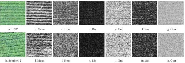
Fig. 3 Spatial distribution of GLCM texture features extracted from Sentinel-2 and UAV imagery during a typical soybean growth stage |
Based on the synthesized half-monthly and monthly temporal data, seven vegetation index features closely related to yield were selected. Using temporal remote sensing images, these seven vegetation indices were calculated for each image in ENVI 5.6, serving as an important data foundation for constructing time-series multi-feature images.
1.4 Feature fusion methods for UAV-Sentinel-2 imagery
1.4.1 Transfer learning fusion algorithm
In this study, data fusion was accomplished at the vegetation index-texture-feature layer: the band, vegetation index and texture feature sets of UAV and Sentinel-2 were generated separately first, followed by spatial alignment at the semi-monthly/monthly scale via Transfer Component Analysis, Long Short-Term Memory (LSTM) and Gated Recurrent Unit (GRU). This method not only preserved the spectral-structural spatial information but also avoided error amplification caused by resolution mismatch. Transfer learning, as a significant component of machine learning, applied acquired knowledge to new problems for solving them[22]. Its core idea was to achieve knowledge transfer by identifying correlations between new features and original features[23]. Operating on features rather than raw pixels keeps spectral and structural detail intact while sidestepping the error blow-up that often accompanies resolution upscaling. Transfer Component Analysis(TCA) treats UAV features as the source domain and Sentinel-2 features as the target domain. It learns a shared latent subspace by minimising the maximum mean discrepancy (MMD) between the two distributions[24], so that cross-sensor differences are suppressed without discarding yield-relevant signals[25]. A neural network then maps the aligned features to yield, letting the model draw on both the fine spatial detail of UAV imagery and the regional coverage of Sentinel-2.
1.4.2 Recurrent neural network algorithm
Two fusion operators were considered: channel concatenation (Concat) and element-wise addition (Add). Add compressed heterogeneous features into a single vector and tends to blur cross-sensor distinctions; Concat retained every channel, which is preferable when UAV and Sentinel-2 features differed so markedly in spatial grain and spectral layout. Therefore, UAV and Sentinel-2 features depth-wise were stacked at each time step and fed the resulting tensor through a recurrent network. Plain recurrent neural networks(RNNs) suffer from vanishing gradients over long phenological sequences[26]; LSTM[27] avoids this with three gating units-input, forget and output-that regulate how much past information is kept or discarded. In this setting, the forget gate has an extra benefit: it learned how much of the earlier UAV-Sentinel-2 fused state was worth retaining for the current yield prediction, pruning redundant cross-sensor details automatically. Fig. 4 shows the gating structure.
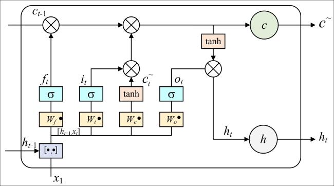
Fig. 4 Diagram of the gate units in an LSTM network |
GRU offers a leaner alternative: only reset and update gates, so parameter count and training time drop noticeably while multi-layer stacks remain feasible. By introducing the reset gate and the update gate, the GRU network can effectively capture both short-term and long-term dependencies in time series. The structural unit of GRU is illustrated in Fig. 5.
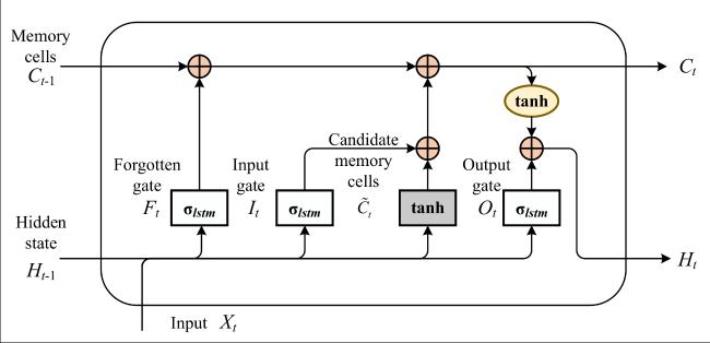
Fig. 5 Diagram of the gate units in the GRU network |
As can be seen from Fig. 5, the inputs to both the reset gate and the update gate of the gating unit are the current time step input and the hidden state from the previous time step. The outputs are obtained through computation by fully connected layers with the Sigmoid activation function. Assuming the number of hidden units is h, the mini-batch input at a given time step t is .
1.5 Improved CNN models
1.5.1 CNN model improved by support vector machine
CNN[28]was a deep-level network structure with nonlinear characteristics, capable of automatically capturing prominent features of soybean vegetation at various levels from remote sensing images. Yet its final fully-connected layers were trained by gradient descent, which was prone to local minima and topology sensitivity. Support Vector Machine(SVM) replaces those layers with a max-margin classifier, so the combined SVM-CNN kept CNN's hierarchical feature extraction while gaining SVM's global convergence and stronger generalisation. In this implementation the CNN trunk stops at its penultimate layer; the deep feature vectors produced there are handed to an SVM for yield regression instead of the usual softmax head. Fig. 6 sketches this architecture.
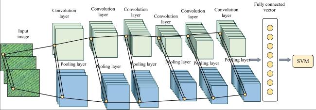
Fig. 6 SVM-CNN model structure diagram |
1.5.2 CNN model improved by attention mechanism
The CNN backbone with two attention plugins was augmented. Squeeze-and-Excitation (SE) attention recalibrates channel importance after each convolution block, boosting bands or indices that carry more yield information. SA attention computes pairwise affinities across the entire temporal sequence, so the model can directly relate distant phenological stages without routing information through recurrent hidden states.Unlike RNNs, Self-Attention (SA) processes the whole sequence in parallel. Every time step is compared against every other via scaled dot-product similarity, and the resulting weights highlight stages most relevant to final yield-pod filling, for instance-regardless of how far apart they are in the growing season. This sidesteps the information bottleneck of recurrent hidden states and trains faster. Fig. 7 depicts the computation.
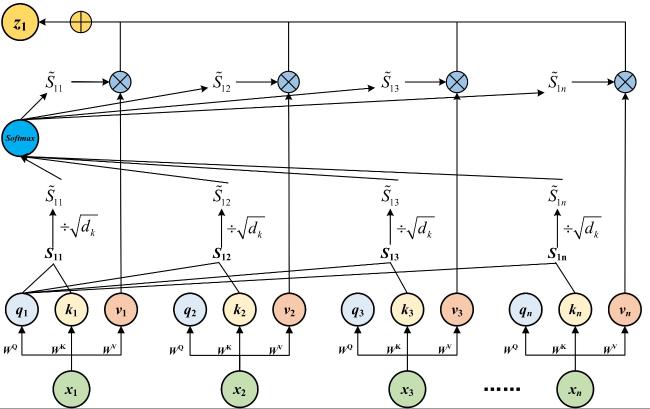
Fig. 7 Calculation process of the self-attention mechanism module |
SE begins by squeezing each feature channel to a single scalar via global average pooling. A tiny fully-connected bottleneck then learns channel-wise dependencies, and the excitation weights are multiplied back to the original feature maps. The whole module is shown in Fig. 8.
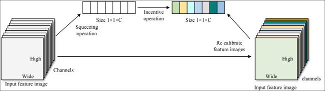
Fig. 8 Schematic diagram of the squeeze-and-excitation (SE) attention mechanism module |
With only 110-130 days of growth[29], the sample windows were short, and the full Transformer would overfit. SA-GRU offers a lighter compromise: about one-sixth the parameters of Transformer-Base[30], yet bidirectional gating and SA recalibration of the 230 fused features still sharpen NDVI gradients and texture cues tied to yield[31]. The full pipeline (Fig. 9) is straightforward: a CNN front-end extracts spatial-spectral features, a pooling layer compresses them, GRU or LSTM models the phenological trajectory, SA highlights critical time steps, and a single output neuron gives the yield estimate.
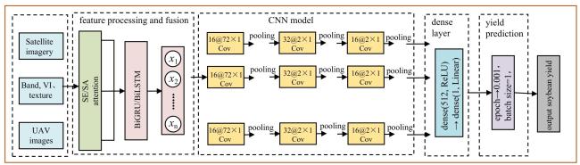
Fig. 9 Structure of CNN-GRU/LSTM-Attention model |
Models were built and trained in MATLAB 2023a. Biases were zero-initialised. Training started at a learning rate of 0.001, decaying to 0.000 1 over 200 epochs via cosine schedule, with the Adam optimiser and batch size 1. The 2022 fused dataset was split 7:3 into training and validation subsets, separately for half-monthly and monthly series. After 1 000 epochs, the checkpoint with the lowest validation loss was kept for testing.
1.6 Feature fusion of multi-source data based on UAV-Sentinel-2
1.6.1 Construction of time series multi-feature imagery
Each input sample was a two-dimensional matrix whose rows were time steps (15-day or 30-day composites) and whose columns were the extracted features. Stacking vegetation-index bands in this way turned a raw time series into an image-like tensor that preserved both phenological progression and spectral state. Neural networks then digest this tensor, learning how soybean canopy signatures evolve and converge on a yield value. The two time-series multi-feature image (TSMFI) sets was constructed. The monthly set holds one composite per month (May-September 2022 and 2023, five images per year); the half-monthly set holds two composites per month, giving ten images per year. The feature depth was 18 for UAV (5 spectral + 6 texture + 7 vegetation indices) and 23 for Sentinel-2 (10 spectral + 6 texture + 7 vegetation indices).
In ENVI 5.6, the Layer Stacking tool was used to extract texture metrics, vegetation indices, and other features from each full-month image (May-September 2022, five scenes in total). The resulting single-band feature images were then sequentially stacked onto the corresponding temporal layer, yielding one full-month time-series multi-feature image whose total band count equals the sum of spectral bands, texture features, and vegetation indices.
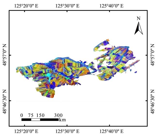
Fig. 10 Multi-feature time-series imagery of Sentinel-2 for the full months of 2022 at Jianshan Farm, Heilongjiang province |
Sampling points were extracted from the composited time series multi-feature images. The field sampling area was divided into grids using the grid method, and within each grid, sampling was conducted using the five-point sampling method. Ground-truth sampling points were overlaid on the TSMFI stack in ArcGIS. A 0.5 m radius around each sample centre (Fig. 11) defined the pixel-extraction window, and all values inside were pooled. Both temporal resolutions were exported to CSV. Before model feeding, the table was reshaped so that every feature (e.g. NDVI) formed a contiguous time vector (May through September), followed by the next feature; this row-major layout makes it easy to trace how any single variable drifts through the season.
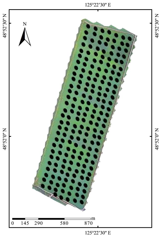
Fig. 11 Sampling point extraction scheme based on ArcGIS at Jianshan Farm |
1.6.2 Feature fusion based on transfer learning algorithms
The TCA algorithm process assumed the existence of a feature mapping space ϕ, where the data exhibited similar distribution characteristics in the mapped feature space. If the marginal distributions of the data were close, the conditional distributions of the two data domains will also be similar. The process began by loading the extracted multi-temporal feature data from UAV and Sentinel-2, followed by invoking TCA to solve for the mapping and conducting tests. The input data consisted of two feature matrices from UAV and Sentinel-2 imagery. The m and H matrices were calculated separately, and a common kernel function (linear or Gaussian) was selected for mapping to obtain K, which then led to the extraction of the top m eigenvalues. X represented the data matrix composed of both source and target domain data, and C denoted the total number of classes. In the UAV and Sentinel-2 feature datasets, the parameters were set as follows: C was the penalty coefficient, set as 10; M denotes the MMD (Maximum Mean Discrepancy) matrix L, which became the global MMD matrix when C=0, and corresponded to a matrix for each class when C was not zero; I was the identity matrix; λ was a fixed balancing parameter; H was the centering matrix, which can be directly calculated; ∅ represented the Lagrange multipliers, which were not directly used in the solution process.
To implement the TCA algorithm using Python 3.8, the specific implementation steps are as follows:
Step 1: The feature data extracted from the UAV serves as the source domain data, while the feature data extracted from Sentinel-2 serves as the target domain data. Xs and Xt were used as the input data for the TCA method.
Step 2: Calculate the L and H matrices, and select an appropriate kernel function to compute K.
Step 3: Adjust the data dimensionality, output the newly aligned source and target domain feature sample sets Ts and Tt after distribution alignment, and verify whether the MMD between the datasets had reached a minimum value. The fusion results are illustrated in Fig. 12.
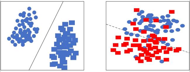
Fig. 12 Feature distribution alignment results of UAV and Sentinel-2 data using TCA algorithma. UAV source domain feature distribution b. Sentinel-2 target domain feature distribution |
1.6.3 UAV-Sentinel-2 time-series feature fusion via LSTM/GRU
RNN-based fusion concatenates UAV and Sentinel-2 feature vectors at every time step. The half-monthly tensor has 230 channels (UAV 18 + Sentinel-2 23, doubled because of the 10 time steps), and the monthly tensor has 115. This part focuses on LSTM and GRU's digestion of this mixed stream. Feature engineering and model training were done in MATLAB 2023a. The raw 230-channel half-monthly input is unwieldy and contains redundant cross-sensor correlations, so it was fed through a combined LSTM-GRU encoder that compresses the stream while preserving the temporal structure most relevant to yield.
(1) Normalization preprocessing is conducted on the input features and labels from UAV and Sentinel-2. To unify the input range of the feature data in the training set, the feature data in the test set undergoes the same transformation as the training set, thereby maintaining consistency.
(2) LSTM/GRU Network Fusion Process. Sliding time window processing was applied to the piecewise linear fitting HI data after normalization. Assuming the feature vector at time t was represented as , where d was the number of input features. Since there was a correlation between the current time window data and historical data, the sliding window method was used to incorporate historical data into the current input data. w represents the window size, which indicated the time length of historical data related to the current data, as shown in Fig. 13.
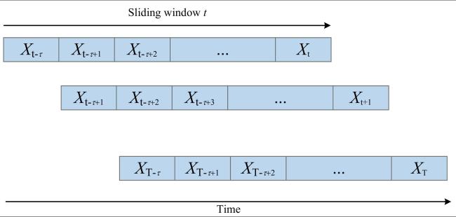
Fig. 13 Sliding time window processing for LSTM/GRU sequential feature fusion |
At each time step of the LSTM/GRU model input, the input features were obtained through sliding time window processing, consisting of input features from the current moment and all historical moments. Starting from time t and up to the point of feature fusion, the time window length L of the sliding window was set to 3. The LSTM/GRU feature fusion process is illustrated in Fig. 14.
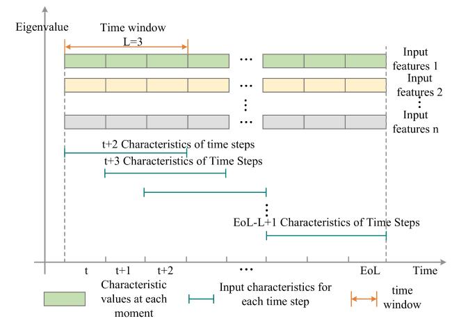
Fig. 14 LSTM/GRU feature fusion process for UAV-Sentinel-2 multi-source data |
2 Results and analysis
2.1 Establishment of soybean yield estimation models using CNN
Under identical CNN hyperparameters, six models were trained: two single-source baselines (CNN-UAV and CNN-Sentinel-2) at half-monthly and monthly scales, and two normalized fusion models (CNN-US). Table 3 reveals three clear patterns. (i) Finer temporal granularity helps: every half-monthly model beat its monthly sibling, especially for Sentinel-2 (R 2 jumps from 0.21 to 0.32). (ii) UAV outperformed Sentinel-2 when used alone at either scale, thanks to its finer ground resolution. (iii) Sensor fusion always won: CNN-US-15 tops the board (R 2=0.44, MAE=21.83 kg/hm2, MAPE=9.57 %), and CNN-US-30 was the best monthly model (R 2=0.40).
Table 3 Performance comparison of CNN yield estimation models using half-monthly and monthly multi-feature time-series data |
| Model | MAE/(kg/hm2) | RMSE/(kg/hm2) | MAPE | R 2 |
|---|---|---|---|---|
| CNN-UAV-15 | 22.294 1 | 30.850 5 | 0.106 6 | 0.39 |
| CNN-Sentinel-15 | 26.461 6 | 32.930 7 | 0.111 6 | 0.32 |
| CNN-US-15 | 21.827 5 | 28.974 6 | 0.095 7 | 0.44 |
| CNN-UAV-30 | 24.895 8 | 31.450 9 | 0.105 8 | 0.37 |
| CNN-Sentinel-30 | 27.005 5 | 34.359 5 | 0.120 5 | 0.21 |
| CNN-US-30 | 22.177 5 | 29.737 7 | 0.096 8 | 0.40 |
|
In terms of overall trends, comparing the half-month temporal data model with the full-month temporal data model revealed that the length of the temporal sequence impacts model performance. The use of half-month phase data performed better in multiple models compared to full-month phase data, as it provided more frequent vegetation information on soybeans, which was more conducive to fine monitoring of vegetation growth changes and thus more accurate capture of data trends. Whether for full-month or half-month multi-feature data, single UAV data outperformed Sentinel-2 predictions, as UAV imagery provides higher spatial resolution and more detailed crop growth information. The models using normalized fused UAV and Sentinel-2 data achieved R 2 values of 0.44 and 0.40 for half-month and full-month fused multi-feature data, respectively, and other indicators were also superior to those of single-data-source models, demonstrating the effectiveness of multi-source data fusion. It indicated that utilizing UAV-Sentinel-2 multi-source data fusion enhanced the accuracy of soybean yield estimation model prediction performance.
2.2 Comparative analysis of multi-source data fusion methods
To further enhance the comprehensiveness and performance of multi-source data fusion, three fusion methods were selected for comparative experiments in this study: normalization, transfer learning, and RNN. The comparison results of CNN models under the three fusion methods are presented in Table 4.
Table 4 Performance comparison of CNN models with different fusion methods for half-monthly and monthly time-series data |
| Model | MAE/(kg/hm2) | RMSE/(kg/hm2) | MAPE | R 2 |
|---|---|---|---|---|
| CNN-US-15 | 21.827 5 | 28.974 6 | 0.095 7 | 0.44 |
| CNN-TCA-15 | 15.172 2 | 18.633 1 | 0.064 3 | 0.88 |
| CNN-GRU-15 | 12.526 8 | 17.254 5 | 0.055 5 | 0.90 |
| CNN-LSTM-15 | 10.093 1 | 14.137 4 | 0.045 0 | 0.93 |
| CNN-US-30 | 22.177 5 | 29.737 7 | 0.096 8 | 0.40 |
| CNN-TCA-30 | 21.568 8 | 27.953 3 | 0.092 6 | 0.71 |
| CNN-GRU-30 | 19.322 2 | 26.188 7 | 0.083 2 | 0.79 |
| CNN-LSTM-30 | 18.030 7 | 25.131 2 | 0.080 7 | 0.80 |
At the half-monthly scale, CNN-LSTM led (R 2=0.93, MAE=10.09 kg/hm2), while CNN-GRU was the best monthly fusion (R 2=0.80). The half-monthly results were markedly stronger across the board because shorter compositing captured canopy dynamics that monthly averaging blurred. Every advanced fusion beat the normalised baseline, but gains differ: LSTM added 0.49 to the half-monthly baseline and 0.40 to the monthly baseline; GRU added 0.46 and 0.39; TCA trailed with 0.44 and 0.31. Recurrent fusion therefore offered the steepest accuracy lift, with LSTM slightly edging GRU at fine temporal resolution.
2.3 Comparative analysis of improved CNN models
To further enhance the prediction performance, three improved CNN models, namely SVM-CNN, SA-CNN, and SE-CNN, were established using data fused by three different methods, respectively. The results of the improved CNN models established using different fusion methods for half-month temporal data are shown in Table 5.
Table 5 Performance of improved CNN models with different fusion methods for half-monthly time-series data |
| Model | MAE/(kg/hm2) | RMSE/(kg/hm2) | MAPE | R 2 |
|---|---|---|---|---|
| SVM-US-CNN | 42.304 6 | 55.776 7 | 0.191 5 | 0.38 |
| SVM-TCA-CNN | 35.184 3 | 45.623 3 | 0.168 3 | 0.66 |
| SVM-GRU-CNN | 31.577 1 | 38.886 2 | 0.153 2 | 0.73 |
| SVM-LSTM-CNN | 26.336 9 | 32.266 6 | 0.132 6 | 0.80 |
| SA-US-CNN | 10.730 5 | 14.740 8 | 0.050 4 | 0.85 |
| SA-TCA-CNN | 9.488 0 | 13.941 9 | 0.048 9 | 0.87 |
| SA-GRU-CNN | 8.403 8 | 12.283 8 | 0.037 8 | 0.94 |
| SA-LSTM-CNN | 10.219 8 | 14.569 3 | 0.0454 | 0.91 |
| SE-US-CNN | 14.983 6 | 12.230 6 | 0.104 2 | 0.70 |
| SE-TCA-CNN | 11.693 5 | 13.983 2 | 0.0963 | 0.71 |
| SE-GRU-CNN | 11.707 1 | 12.191 7 | 0.053 0 | 0.90 |
| SE-LSTM-CNN | 8.520 9 | 12.609 2 | 0.036 8 | 0.92 |
For the SVM-CNN model was enhanced by different fusion techniques, the prediction accuracy of the model gradually increases, with indicators such as MAE, RMSE, and MAPE decreasing progressively. Specifically, MAE decreased from 42.304 6 to 26.336 9, and R 2 rised from 0.38 to 0.80. The SVM-LSTM-CNN model achieves the best R 2 of 0.80. In the case of the SA-CNN model improved by different fusion methods, MAE drops from 10.730 5 to 8.403 8, and R 2 increased from 0.85 to 0.94. The SA-GRU-CNN model performs best, exhibiting the lowest MAE (8.403 8) and the highest R 2 (0.94). The results of the improved SE-CNN model remained stable across various fusion methods, with MAE decreasing from 14.983 6 to 8.520 9 and R 2 increasing from 0.70 to 0.92. The SE-LSTM-CNN model performs optimally, featuring the lowest MAE (8.520 9) and the highest R 2 (0.92). Both the SA-CNN and SE-CNN models demonstrate lower prediction errors than the SVM-CNN in all scenarios. GRU and LSTM perform better across all models because they can better capture the bidirectional dependencies in time series data. In summary, the best model for half-monthly time series accuracy is the SA-GRU-CNN, with an R 2 of 0.94.
After applying three fusion methods to multi-feature monthly time series data, three improved CNN models were established. The results of these improved CNN models, which were built using different fusion methods for monthly time series, are presented in Table 6.
Table 6 Performance of improved CNN models with different fusion methods for monthly time-series data |
| Model | MAE/(kg/hm2) | RMSE/(kg/hm2) | MAPE | R 2 |
|---|---|---|---|---|
| SVM-US-CNN | 48.918 5 | 58.501 2 | 0.211 0 | 0.25 |
| SVM-TCA-CNN | 45.172 2 | 56.643 1 | 0.189 9 | 0.58 |
| SVM-GRU-CNN | 41.448 2 | 55.486 7 | 0.173 6 | 0.69 |
| SVM-LSTM-CNN | 28.893 5 | 36.069 6 | 0.152 6 | 0.79 |
| SA-US-CNN | 10.524 5 | 14.188 6 | 0.048 1 | 0.83 |
| SA-TCA-CNN | 7.777 5 | 10.654 0 | 0.035 5 | 0.86 |
| SA-GRU-CNN | 12.201 6 | 17.046 4 | 0.052 0 | 0.91 |
| SA-LSTM-CNN | 12.183 3 | 17.698 3 | 0.052 4 | 0.90 |
| SE-US-CNN | 14.974 6 | 32.250 4 | 0.108 2 | 0.66 |
| SE-TCA-CNN | 11.568 8 | 25.953 3 | 0.083 2 | 0.71 |
| SE-GRU-CNN | 17.902 1 | 25.219 7 | 0.076 3 | 0.78 |
| SE-LSTM-CNN | 14.953 4 | 20.938 2 | 0.063 8 | 0.85 |
In Table 6, among all the improved methods, Across all four fusion configurations (US, TCA, GRU, LSTM), the corresponding SA-CNN and SE-CNN variants consistently outperformed their SVM-CNN counterparts. For instance, under the US fusion method, SA-CNN and SE-CNN achieved R 2 values of 0.83 and 0.66, respectively, far exceeding the 0.25 of SVM-CNN; under the LSTM fusion method, the three models attained R 2 of 0.90, 0.85, and 0.79, respectively. This indicated that the attention mechanism (SA/SE) was more effective than SVM in enhancing CNN-based yield estimation. For the improved SVM-CNN model, when using the US method, the MAE is 48.918 5 and the RMSE is 58.501 2, indicating significant prediction errors. The R 2 value of 0.25 suggests a low degree of fit of the model to the data. As the complexity of the fusion methods increases (from TCA to LSTM), both MAE and RMSE gradually decrease, while the R 2 value gradually increases. The SVM-LSTM-CNN model performs best, with MAE reduced to 28.893 5 and R2 increased to 0.79. For the SA-CNN model, using only the normalization fusion method already demonstrates high prediction accuracy (MAE=10.524 5, RMSE=14.188 6, R 2=0.83). Under the TCA fusion method, MAE drops to 7.777 5 and R² rises to 0.86. The SA-GRU-CNN model achieves the best R 2 of 0.91. For the SE-CNN model, when using the normalization fusion method, the prediction errors are MAE=14.974 6, RMSE=32.250 4, and R 2=0.66. The SE-LSTM-CNN model achieves the best R 2 of 0.85. In summary, for the monthly time series dataset, the SA-GRU-CNN model performs best with the highest accuracy of 0.91.
SA-GRU-CNN wins at both scales (R 2= 0.94 and 0.91). The SA module highlights yield-critical time steps, while GRU preserves long-range phenological memory; together they extract more predictive structure than either mechanism alone. The 0.03 drop from half-monthly to monthly is modest but consistent, reaffirming that half-monthly revisits are preferable for this crop and region. An ablation study was run to isolate the contribution of each design choice. Starting from plain CNN-UAV, US fusion, SG smoothing, GRU, and SA were added successively, training a separate model at every stage. As shown in Table 7, with the gradual addition of key modules, the yield estimation accuracy has continuously improved.
Table 7 Ablation study results of the SA-GRU-CNN model on half-monthly time-series data |
| Model | R 2 | MAE/(kg/hm2) | RMSE/(kg/hm2) | MAPE |
|---|---|---|---|---|
| UAV-CNN | 0.37 | 24.90 | 31.45 | 0.106 |
| US-CNN fusion | 0.44 | 21.83 | 28.97 | 0.096 |
| SG-CNN | 0.71 | 15.17 | 18.63 | 0.064 |
| GRU-CNN | 0.90 | 12.53 | 17.25 | 0.056 |
| SA-GRU-CNN | 0.94 | 8.40 | 12.28 | 0.038 |
The sequential ablation in Table 7 tracked performance as modules are cumulatively added: UAV-CNN (R 2=0.37) → US fusion (Δ R 2 +0.07) → SG filtering (Δ R 2 +0.27) → GRU (Δ R 2 +0.19) → SA attention (Δ R 2 +0.04), reaching 0.94. While this design did not isolate individual module effects (e.g., GRU's contribution was confounded with SG filtering), the stepwise Δ R2 suggested that SG temporal smoothing and GRU sequential modeling provide the largest marginal gains. SA's contribution, though positive, was comparatively modest. A more rigorous ablation would require evaluating each module independently and in reverse-removal configurations to establish true indispensability.
2.4 Yield analysis of the optimal soybean yield estimation model
Based on the yield prediction results from the best half-monthly SA-GRU-CNN model in 2022, the yields for Fields 13, 14, and 15 in the north were 3 075 kg/hm2, 3 090 kg/hm2, and 3 255 kg/hm2, respectively; while the actual harvested yields were 3 180 kg/hm2, 3 255 kg/hm2, and 3 375 kg/hm2, respectively. The corresponding relative errors were 3.30% (North 13 Plot), 5.07% (North 14 Plot), and 3.56% (North 15 Plot), yielding a mean absolute percentage error (MAPE) of 3.98% across the three plots. The predicted yield information along with their corresponding latitude and longitude coordinates were imported into ArcGIS 10.6, using the Kriging interpolation algorithm, a yield distribution map (Fig. 15) for Fields 13, 14, and 15 in the north of Jianshan Farm was created, visually displaying the spatial distribution of soybean yields.
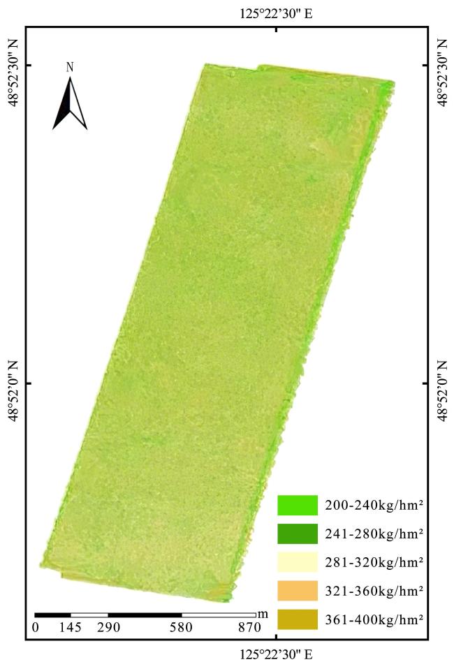
Fig. 15 Spatial distribution of predicted soybean yield for North 13, 14 and 15 Plots at Jianshan Farm in 2022 |
2.5 Validation of the optimal yield estimation model
Given that the results above indicated, only half-monthly time series data for 2023 was validated. Using the soybean yield estimation model for 2022, predictions were made based on the remote sensing data for 2023. The prediction results of the improved CNN models with different fusion methods for 2023 half-monthly time-series soybean yield estimation at Jianshan Farm are presented in Table 8.
Table 8 Performance of improved CNN models with different fusion methods for half-monthly time-series data in 2023 |
| Model | MAE//(kg/hm2) | RMSE/(kg/hm2) | MAPE | R 2 |
|---|---|---|---|---|
| SVM-US-CNN | 43.456 2 | 55.967 5 | 0.196 6 | 0.37 |
| SVM-TCA-CNN | 34.683 2 | 44.326 8 | 0.153 4 | 0.67 |
| SVM-GRU-CNN | 31.867 4 | 39.326 5 | 0.157 6 | 0.72 |
| SVM-LSTM-CNN | 26.635 9 | 31.324 4 | 0.113 5 | 0.81 |
| SA-US-CNN | 15.786 5 | 14.964 2 | 0.056 8 | 0.84 |
| SA-TCA-CNN | 9.569 0 | 13.082 6 | 0.040 9 | 0.86 |
| SA-GRU-CNN | 8.253 8 | 9.603 9 | 0.036 5 | 0.93 |
| SA-LSTM-CNN | 16.326 5 | 15.834 5 | 0.073 2 | 0.82 |
| SE-US-CNN | 14.504 9 | 12.130 9 | 0.103 3 | 0.71 |
| SE-TCA-CNN | 10.236 9 | 12.026 0 | 0.086 3 | 0.73 |
| SE-GRU-CNN | 8.962 3 | 11.160 2 | 0.070 9 | 0.79 |
| SE-LSTM-CNN | 8.054 2 | 9.863 4 | 0.059 6 | 0.91 |
In table 10, the SVM-CNN model shows poor prediction performance for the half-monthly time series. The improved SA-CNN model demonstrates good prediction performance, with the SA-GRU-CNN model achieving the best results, boasting the highest R 2 value of 0.93. Among the improved SE-CNN models, the SE-BiLSTM-CNN model performs best, with the highest R 2 value of 0.91. Prediction results from both years consistently indicate that the SA-GRU-CNN model exhibits the best performance in predicting soybean yields.
2.6 Discussions
Field data from 2022 and 2023 confirmed that fusing UAV and Sentinel-2 data is viable for regional soybean yield mapping. SA-GRU-CNN scored R 2=0.94 on the 2022 half-monthly set and R 2=0.93 on the independent 2023 set, so the pipeline is stable across growing seasons. These results were discussed below, and this design choices were compared with recent literature on multi-source crop yield estimation.
Recurrent fusion (LSTM/GRU, R 2= 0.90~0.93) outperforms TCA alignment (R 2=0.88) because gates learn dynamic phenological complementarity rather than forcing a static shared subspace. LIAO et al.[5] report a similar gap: their Landsat-MODIS temporal fusion for maize and soybean stalled at R 2= 0.84, partly because Landsat-MODIS blending cannot recover cloud-induced gaps or growth-stage lag. This UAV-Sentinel-2 pairing sidesteps both problems: UAV fills local texture detail, while Sentinel-2 provides regional spectral coverage. YANG et al.[7], fusing only UAV sensors (RGB-MS-TIR), reached R 2=0.66 on wheat-much lower than this scores-underscoring that cross-platform fusion outclasses single-platform sensor stacking when spatial scale and spectral breadth differ so widely.
The three-point accuracy gain from monthly to half-monthly (R 2= 0.91 vs. 0.94) is ecologically grounded. Soybean's yield-critical window (R3-R6) spans only 30~40 days; half-monthly compositing catches the rapid NDVI rise and any mid-season stress dip, whereas monthly averaging smears these short-lived signals. SGFA with a half-monthly window and third-order polynomial keeps the curve smooth yet retains the key inflection points-a trade-off validated by Candan's cross-validation work on polynomial order[32]. One remaining weak spot is temporal matching: UAV and Sentinel-2 passes were aligned manually, and cloudy slots (notably July-August rains in Heilongjiang) were therefore prone to misalignment.That misalignment likely inflates the monthly MAE because a single bad match affects a larger time block. However, the current temporal matching strategy relies on manual alignment of the overpass dates of UAV and Sentinel-2, which may lead to temporal misalignment in cloudy regions (e.g., the rainy season from July to August in Heilongjiang Province). This is an important reason for the relatively high MAE of monthly data.
3 Conclusions
The research is based on the multi-source data fusion, integrating UAV and Sentinel-2 remote sensing imagery to develop an improved deep learning model for predicting soybean yields. Field data and remote sensing data were collected from Jianshan Farm, and preprocessing and feature extraction of the remote sensing imagery was conducted. Soybean yield estimation models based on multi-scale spatial feature fusion of UAV-Sentinel-2 imagery were established, and soybean yield estimation models using three improved CNN were proposed. The main conclusions are as follows:
(1) SGFA-based compositing at half-monthly and monthly scales effectively bridges the temporal-spatial gap between UAV and Sentinel-2 imagery. From 124 Sentinel-2 scenes and 47 UAV flights, Spectral, textural, and vegetation-index features were extracted to build time-series multi-feature datasets, which resolved resolution mismatches between the two sensors.
(2) Multi-source fusion consistently surpassed single-source modelling. At the half-monthly scale, the CNN-LSTM strategy attained the highest accuracy (R 2=0.93), indicating that LSTM gating was well suited to sequential remote-sensing features.
(3) Validation against 2023 data confirms the stability of these results: the SA-GRU-CNN model again reaches R 2=0.93 on half-monthly series, while transfer-learning fusion lags behind in both years. This reproducibility suggests the framework is robust across growing seasons.
Future work could enrich model inputs with meteorological and soil variables to improve interpretability under abnormal weather, extend the pipeline to maize or wheat to test cross-crop generality, adopt Transformer or Vision Transformer (ViT) modules to exploit fine-grained UAV spatial detail, move from static prediction to real-time forecasting via online learning, and incorporate Landsat-9 or Gaofen-6 imagery to widen the spatial coverage from field to regional/national scales.


